SIRAH Tools GUI

Note

Please report bugs, errors or enhancement requests through Issue Tracker or if you have a question about SIRAH open a New Discussion.

Overview

SIRAH Tools GUI is a user-friendly interface that combines VMD and Python scripts for molecular dynamics (MD) simulation analysis. The main purpose of SIRAH Tools GUI is to aid the analysis of coarse-grained (CG) SIRAH force field MD simulations, providing users with the most widely used trajectory analyses based on VMD syntax and operations without the need of familiarity with its scripting language.

Note

Some of SIRAH Tools GUI features are not specific to CG or SIRAH force field nomenclature. As a result, it is applicable to any MD simulation that makes use of VMD-compatible topology and trajectory files.

The GUI should be easy to use for people who are proficient in both VMD and MD. For beginners, SIRAH Tools GUI is an ideal tool, helping them get past the first learning curve that most MD visualization software imposes.

In addition, it was constructed in a modular manner, combining TCL (.tcl) and Python (.py) scripts (Figure 1), enabling all users to customize the scripts without changing its code.

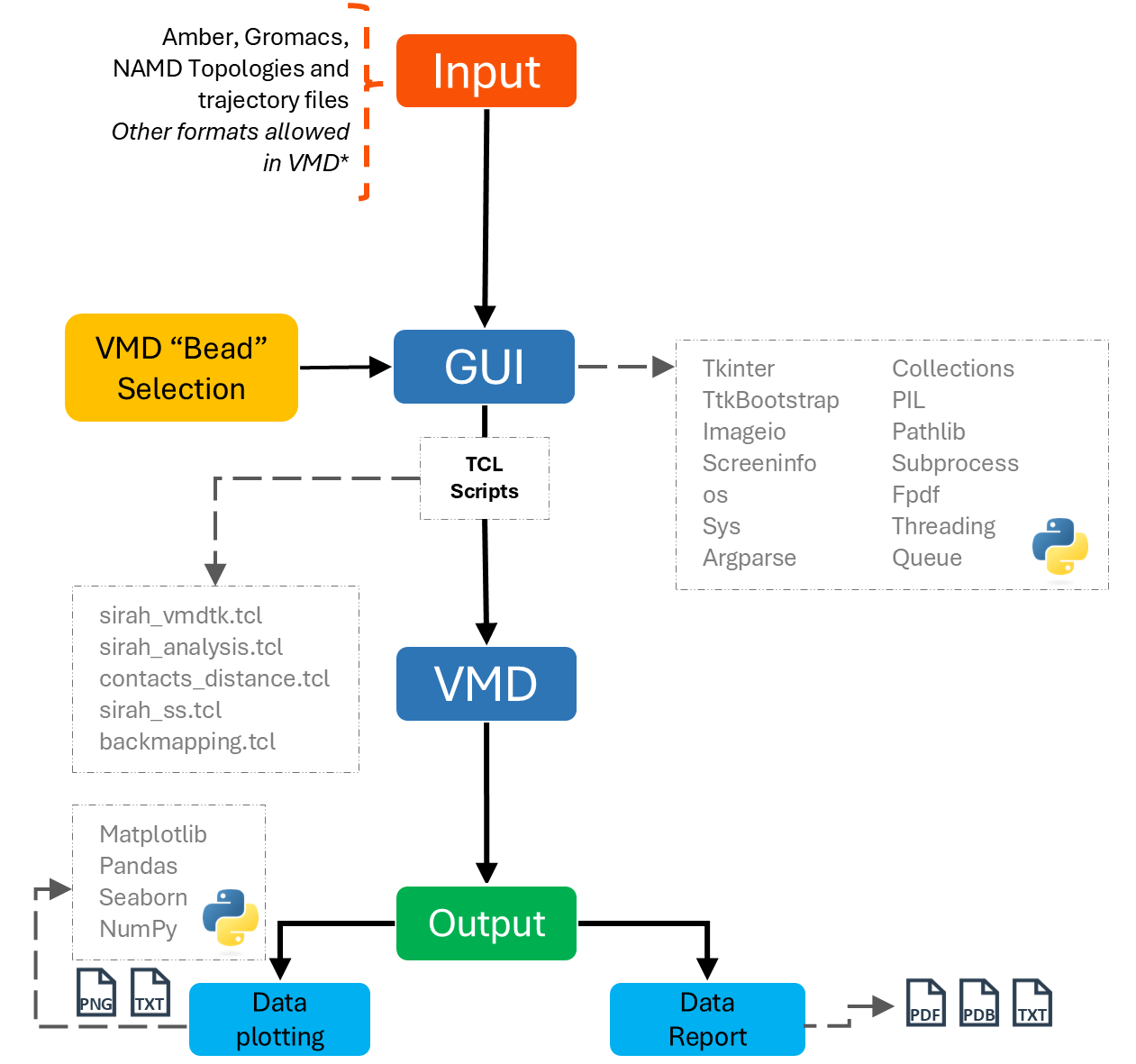
Figure 1. SIRAH Tools GUI organization.

Installing

The environment.yml provided defines all Python dependencies and modules required by SIRAH Tools GUI:

• Python interpreter - python=3.11.5 - (alternative: python=3.10.15)

• Conda packages - numpy=1.24.3 - pandas=2.0.3 - matplotlib=3.7.2 - seaborn=0.12.2 - tqdm=4.65.0

• pip-installed modules - ttkbootstrap==1.10.1 — enhanced GUI styling - fpdf==1.7.2 — PDF report generation - imageio==2.35.1 — image and GIF creation - screeninfo==0.8 — screen-resolution detection - seaborn==0.12.2 — ensures consistent seaborn version

These dependencies guarantee compatibility and stability across all SIRAH Tools GUI features.

1. Clone the Repository:

git clone https://github.com/SIRAHFF/SIRAH-Tools-GUI.git

cd SIRAH-Tools-GUI/

Unzip file:

unzip SIRAH-Tools-GUI_v1.0.zip

cd SIRAH-Tools-GUI_v1.0/

2. Create the Conda Environment:

conda env create -f env_sirah_tools.yml

Activate the Environment:

conda activate sirah-gui

check python version:

python --version

3. Run the aplication:

python sirah-tools-gui.py

The GUI should launch, allowing you to access all the features.

Optional (Advised): Create an Alias

To simplify usage, add an alias in your shell configuration file (e.g., ~/.bashrc or ~/.zshrc):

alias sirah-gui="conda activate sirah-gui && python ``/path/to/SIRAH-Tools-GUI/sirah-tools-gui.py``

Be sure to set /path/to/SIRAH-Tools-GUI/sirah-tools-gui.py to the right path on your computer.

After reloading your shell, simply run:

sirah-gui

If everything went as planned, you should be able to launch the SIRAH Tools GUI interface (Figure 2) and use all of its features.

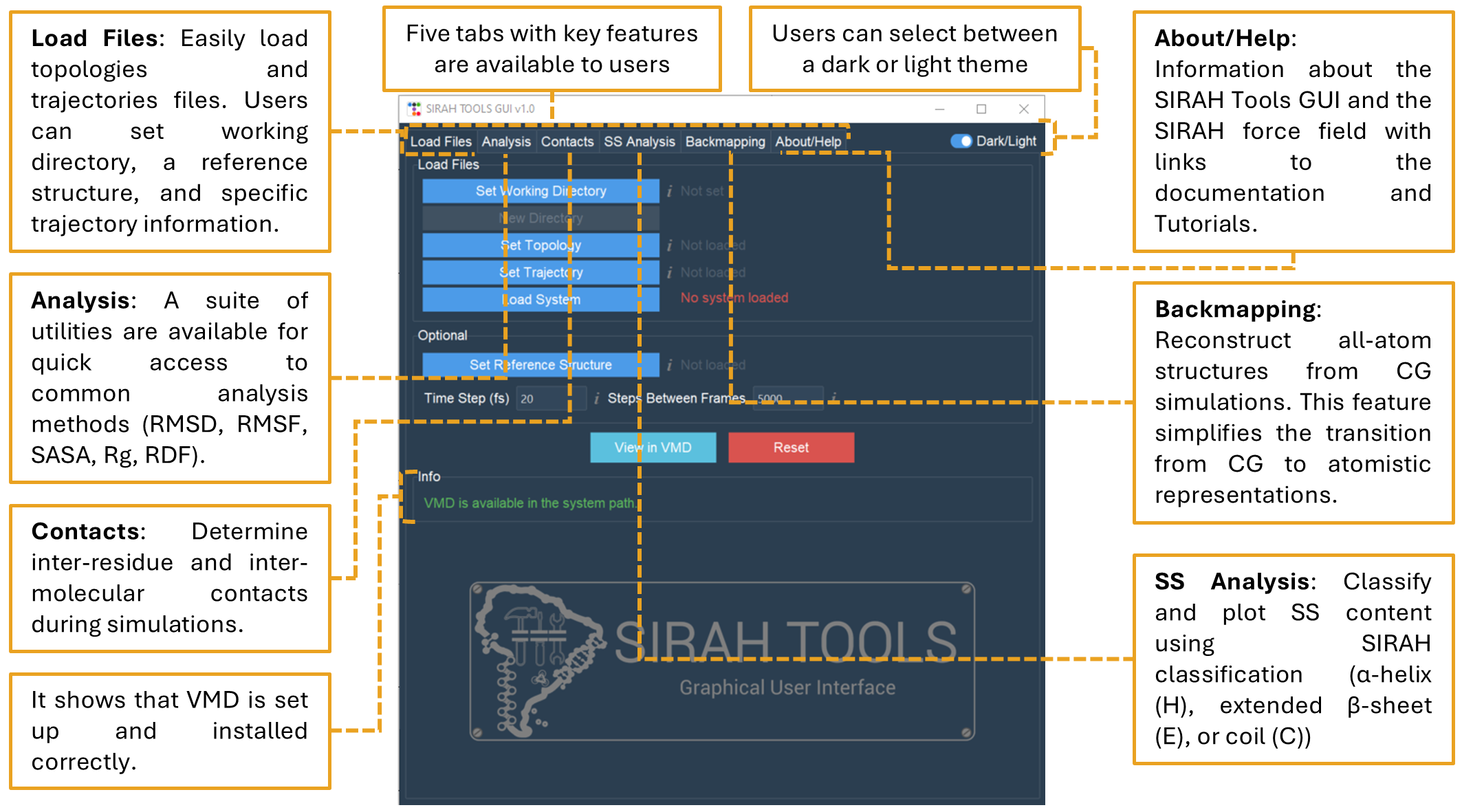
Figure 2. SIRAH Tools Graphical User Interface (GUI) screen to perform MD simulation analysis. It contains five tabs that carry out various analyses and tasks.

Note

SIRAH Tools GUI automatically detects if VMD is set in the system path, this is essential for the correct operation of SIRAH Tools GUI. If VMD is not set up correctly, a warning will be displayed and the tabs will be disabled.

Example of how to use

This example shows how to analyze trajectory files using SIRAH Tools GUI. The main reference for this example are Ballesteros-Casallas et al [Manuscript in Preparation] and Machado & Pantano. The Nucleosome Core Particle (NCP) used here was previously discussed by Brandner et al and Cantero et al. We strongly advise you to read these articles before starting this tutorial.

Warning

Before you can use SIRAH Tools GUI, trajectory files need to be prepared to take into account Periodic Boundary Conditions (PBC). For examples of how to do this, see Amber, GROMACS, or NAMD tutorials.

Note

Apart from the “Load Files” tab that needs to be the first tab, the other tabs don’t need to follow an order. This means that the user can choose any of the tabs to do analysis without having to go through the others.

Loading Files tab

The Load Files tab allows loading AMBER, GROMACS, and NAMD simulation topologies and trajectories compatible with SIRAH force field MD simulations. See more details of the tab here.

Note

The SIRAH Tools GUI works with VMD in text mode; therefore, it can be used on any system that can be loaded in VMD.

Warning

Windows may not support AMBER trajectories in NetCDF format (limited by VMD).

Let’s begin the example by using the SIRAH Tools GUI to open the NCP topology and trajectory files.

Note

Here, the NCP trajectory file was processed to take into account Periodic Boundary Conditions (PBC) and solvent molecules (WT4 beads) were removed. This was done using tools outside SIRAH Tools GUI. For examples of how to do this, look at the Amber, GROMACS, or NAMD tutorials [create links].

First, set up the working directory. This will turn the button green and the path of the chosen directory will be displayed beside it (Figure 3A). All files created will be stored in the working directory.

Warning

Be sure that you selected a folder where you have permission to create and save files.

This will also enable the “New Directory” button (Figure 3A).

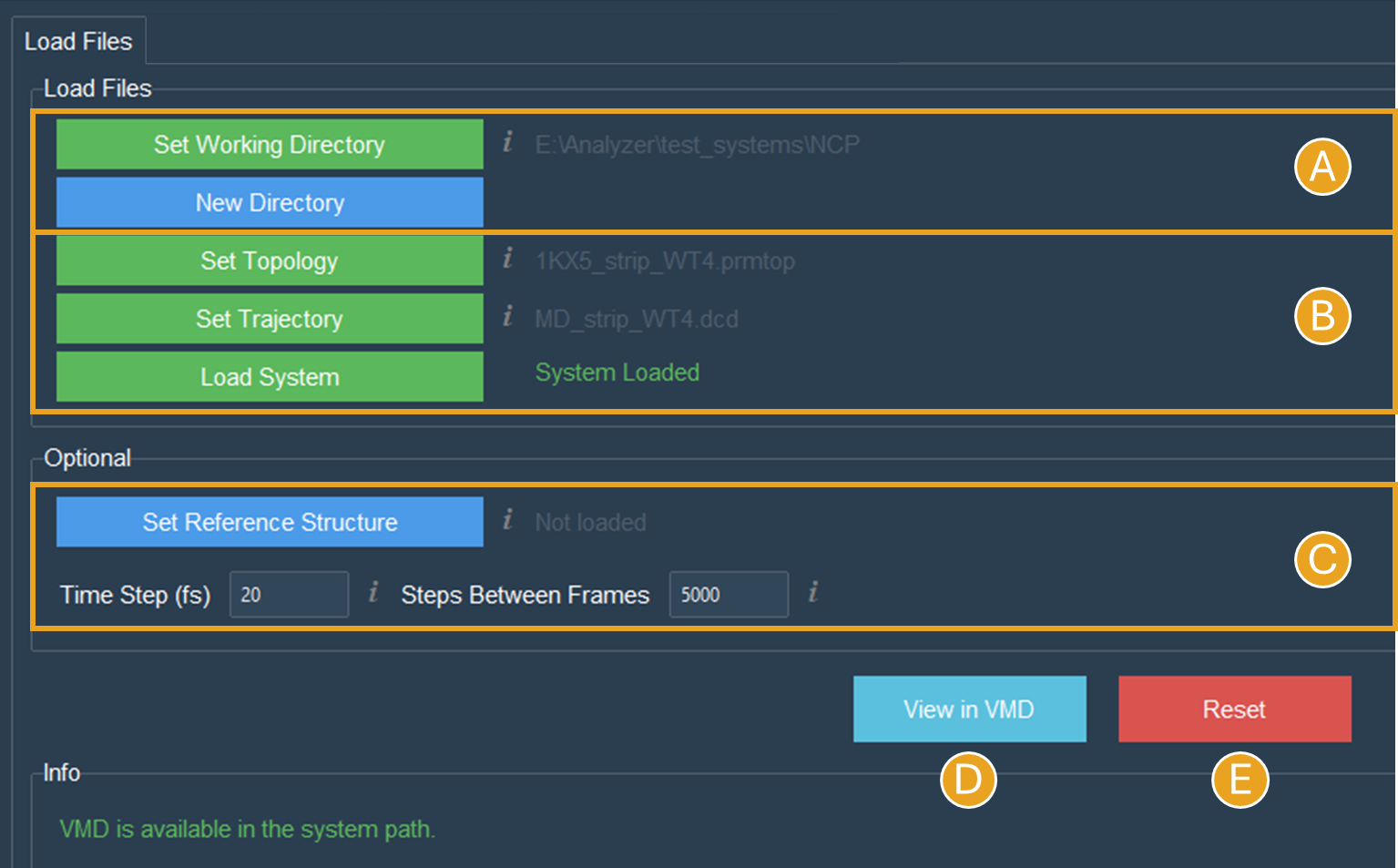
Figure 3. The Load Files tab will appear like this after the topology and trajectory files have been set up and loaded. A) The first step to successfully use SIRAH Tools GUI is to set the working directory. B) The system must be loaded using the “Load System” button after the working directory has been set and the topology and trajectory files have been selected. C) No reference structure was imported, and the options “Time step” and “Step between frames” were set to the default values. D) The “View in VMD” button launches VMD with the loaded system. E) The “Reset” button will erase all data loaded.

Tip

Although it is optional, creating a new directory can help organize the working folder if it contains a lot of files.

Now, click the corresponding buttons to select the topology file and then the trajectory file. This will turn the buttons green and enable the “Load System” button. To load the files, click the “Load System” button. Beside the button, a “System Load” message will appear (Figure 3B).

For this tutorial, no reference file will be imported, and the options “Time step” and “Step between frames” will remain set to the default values used in SIRAH tutorials (since these values were used in the simulation) (Figure 3C).

Note

If different values of “Time step” and “Step between frames” have been applied, users must set them to the appropriate values used in their simulation to make sure the analyses and plots are performed correctly.

If all went well, you should be able to click the “View in VMD” button (Figure 3D) to launch VMD and load the system (Figure 4).

Tip

Although it is not required, visualizing the system in VMD can assist in determining whether any loading issues occurred before beginning any analysis.

Note

Any data entered in the tab will be erased if the “Reset” button (Figure 3E) is clicked.

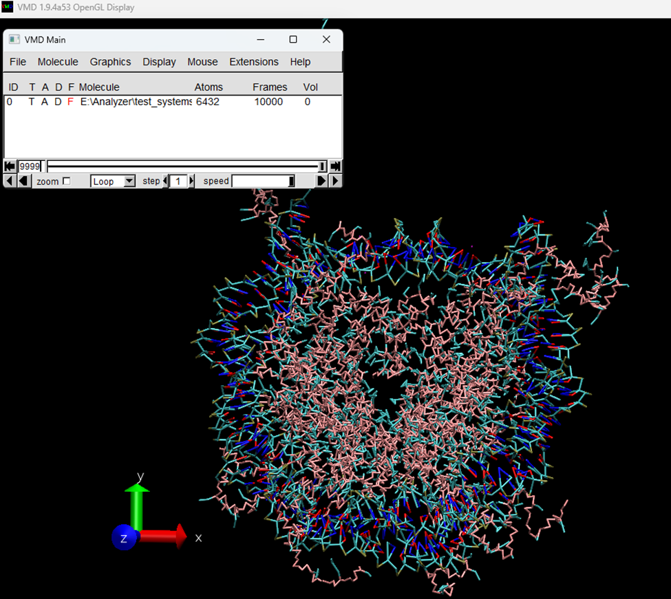
Figure 4. System loaded in VMD using the button ‘View in VMD’. Once the files are loaded correctly, we are ready to start the analysis.

Upon loading the topology and trajectory information, we can start exploring SIRAH Tools GUI’s available analysis.

Basic and Advanced MD Analyses

Here let’s select the Analysis tab. This tab allows several types of MD simulation analysis using VMD syntax selections (e.g. name, resname, resid, etc.) or VMD macros. See more details of the tab here.

Tip

Check out the SIRAH Tools tutorial to learn more about VMD and SIRAH macros and how to use them.

Note

The “Analyze” button will only be enabled if one or more options are selected in either the Basic Analysis or Advanced Analysis sections, but you are not required to check every checkbox.

For the Basic Analysis section, write “name GC or name PX” at the Selection box. Then check the boxes for RMSD, RMSF, and Radius of Gyration (RGYR) (Figure 5A).

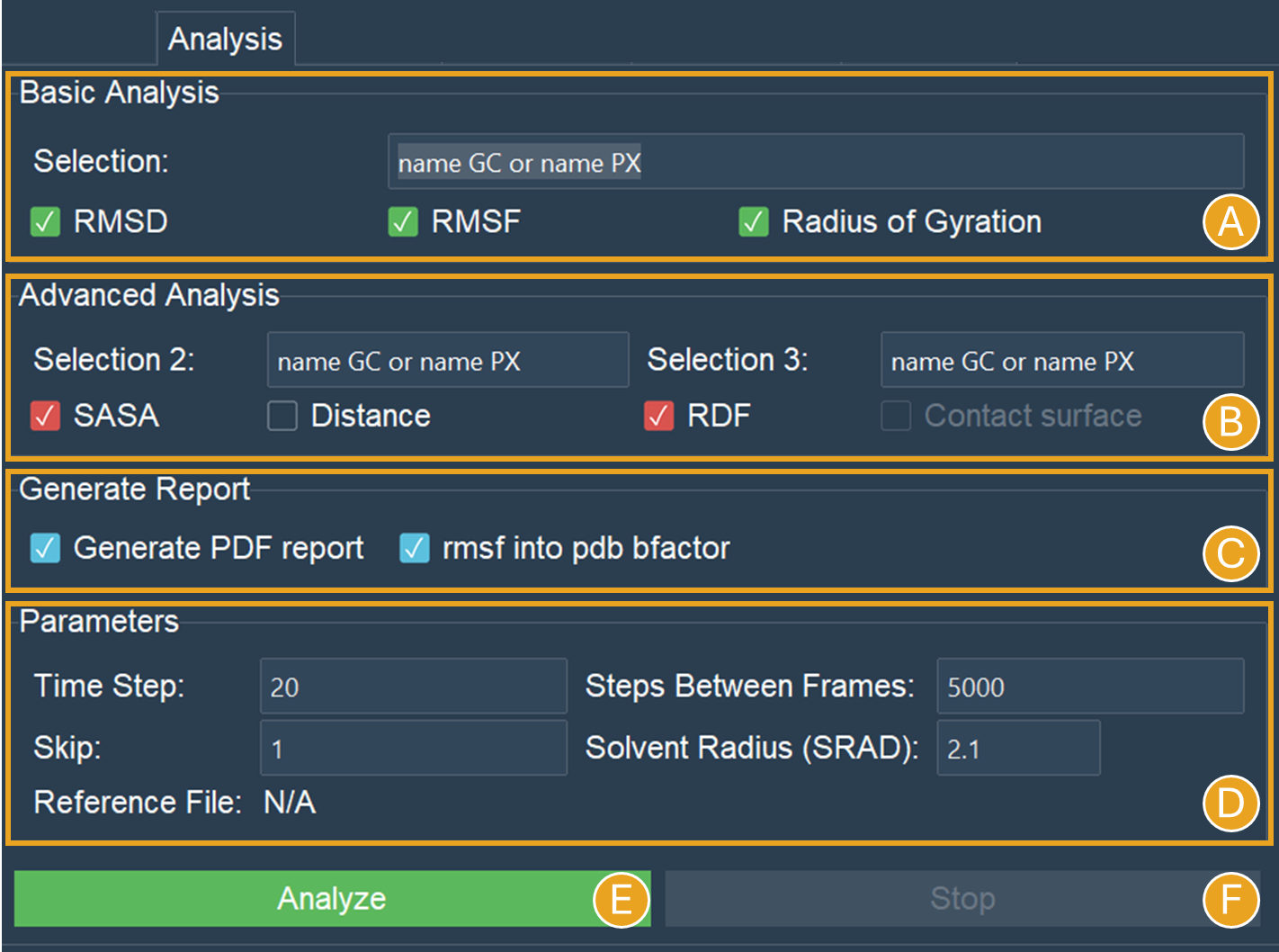
Figure 5. Analysis tab settings for analyses using “name GC or name PX” beads. A) Basic Analysis selection for the NCP system. B) Advanced Analysis selection for the NCP system. C) Selected options in the “Generate Report” section. D) No reference structure was imported, and the options “Time step” and “Step between frames” were set to the default values. However, a 10 frame skip was used. E) The “Analyze” button will perform all the selected actions. F) Only when an analysis is underway is the “Stop” button activated, and pressing it will halt the analysis’s progress.

Tip

Because the NCP simulation has proteins and DNA molecules, we can make a selection for both. The GC bead in SIRAH would be comparable to a protein carbon alpha atom and the PX bead would be comparable to a DNA phosphate atom.

For the Advanced Analysis section, let’s also write “name GC or name PX” next to both Selection 2 and Selection 3, and then check the boxes for SASA and RDF (Figure 5B).

Warning

It is necessary to fill out both selections in the “Advanced Analysis”. This is because the VMD command being used here uses specific flags depending on the analyses. The selections in both boxes may be identical or different. For further information, please see the Developers notes’ information about the Analysis tab here.

Note

All the analyses are selected except “Distance”. This is because “Distance” can only be found between two distinct selections (two distinct beads, two distinct residues, two distinct molecules, etc). Choosing “name GC or name PX” in both boxes will give a zero distance because it is the same group of beads.

For the Generate Report section, check both Generate PDF report and rmsf into pdb bfactor (Figure 5C).

Note

The PDB file generated here uses the first frame coordinates of the beads.

Lastly, let’s give the trajectory a 10-frame “Skip” in the “Parameters” section (Figure 5D). This will speed up the calculations and reduce the number of frames from 10.000 to 1.000. Since the NCP simulation used these “Time step” and “Step between frames” values, leave them at their default settings.

Note

If different values of “Time step” and “Step between frames” have been applied in the MD simulation, users must set them to the appropriate values used in their simulation to make sure the analyses and plots are performed correctly.

Click on the “Analyze” button now that it’s enabled (Figure 5E). A pop-up window indicating that the calculation is running will be shown. Optionally, if required, you can stop the calculation using the “Stop” button (Figure 5F).

Tip

The VMD output area displays information about the VMD execution (as in a terminal window). Thus, any problem or error within the VMD will appear here.

Once the calculation is complete a new folder Analysis is generated in the working directory.

In this example 13 files are generated into this folder. These correspond to the .dat files and the plots (.png files, ploted with python) of RMSD, RMSF, SASA, RGYR, RDF and its integral. The remaining files include the PDF report containing the plots of all analyses and a PDB file (RMSF_protein.pdb) with the RMSF values in the Beta factor column.

Note

The way that the files are named (Name of the Analysis_selection1_selection2.dat or Name of the Analysis_selection1_selection2.png) facilitates the study of various selections in the same folder. New files are created by different selections, whereas files are rewritten over if the same selection is made again. Nevertheless, a pop-up box will question if the user wants to rewrite the files.

Some of the plots produced by the chosen analyses of the “Analysis” Tab are displayed in Figure 6.

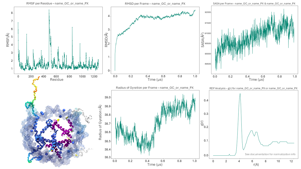
Figure 6. The “Analysis” tab’s outputs include a PDB file, RMSF, RMSD, SASA, RGYR, and RDF plots.

Tip

Any external plotting software or script should be able to use the .dat files. Additionally, the appearance of the plots can be enhanced by adjusting the plot functions (such as plot_generic, plot_rmsf, etc.) in the Python script (/modules/analysis_tab.py).

Calculating Intermolecular and Intramolecular Contacts

Here let’s select the Contacts tab. This tab allows the analysis of contacts between two selections, using VMD syntax selections (e.g. name, resname, resid, etc.) or VMD macros, using a cutoff distance as a criterion. See more details of the tab here.

To better understand the contact tab, let’s split the example into two sections: Intermolecular contacts and Intramolecular contacts.

Intermolecular contacts

To calculate intermolecular contacts, the choices must be in different molecules. For the NCP trajectory, let’s designate Selection1 “name GC”, which gives us the backbone beads (GC) of the histone octamer, and Selection2 “name PX”, which gives us the DNA phosphate beads (Figure 7A).

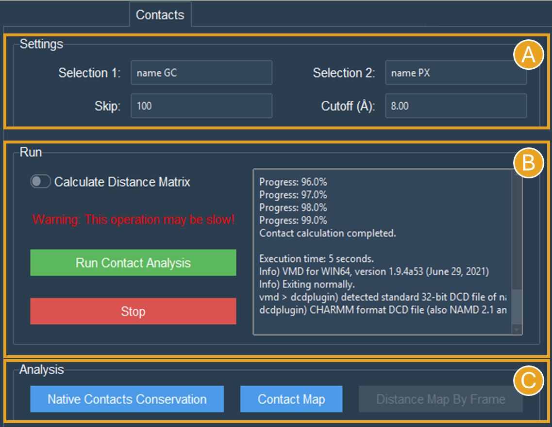
Figure 7. “Contacts” tab settings for intermolecular contacts analyses for the two selections “name GC” and “name PX” beads of the NCP system. A) Settings to contact analysis. Two selections are needed, these selections can be in the same or different molecules. Here, we are using selections from different molecules. The default numbers were set to speed up the calculation. B) Run contacts calculation. A distance matrix can also be calculated. Calculation progress will be displayed and can be stopped at any time. C) When the calculations are done, buttons to make the plots will become active.

Let’s leave the cutoff distance at default value of 8.00 Å and use a 100-frame skip (reducing the 10.000-frame long trajectory to 100 frames) (Figure 7A).

Caution

Keep in mind that the calculation will take longer if the selections have many beads or atoms or if there are a high number of frames to be processed, so be patient.

Leave the Calculate Distance Matrix unselected (Figure 7B) since the matrix here is asymmetric as a result of the varying quantities of GC beads on the histone backbone and PX beads on the DNA phosphates. This asymmetry is expected whenever the two interacting groups are of different sizes, which is typically the case in intermolecular contact analyses.

Click the “Run Contact Analysis” button (Figure 7B).

Tip

The VMD output area will display the progress of the calculation. The calculation can be stopped using the “Stop” button if something goes wrong.

Once the calculation is complete a new folder Contacts is generated in the working directory. To aid in the creation of the contact plots, the “contact length”, “distance length”, “contacts”, “percentage”, and “timeline” .dat files will be created.

Buttons for creating Native Contacts Conservation and Contact Map plots will become active once the calculation is finished (Figure 7C).

Note

The Distance Map By Frame was not activated since no distance matrix was computed.

By clicking on the “Native Contacts Conservation” button, a plot of the conservation of the initial frame contacts between the selections during the simulation can be obtained (Figure 8A).

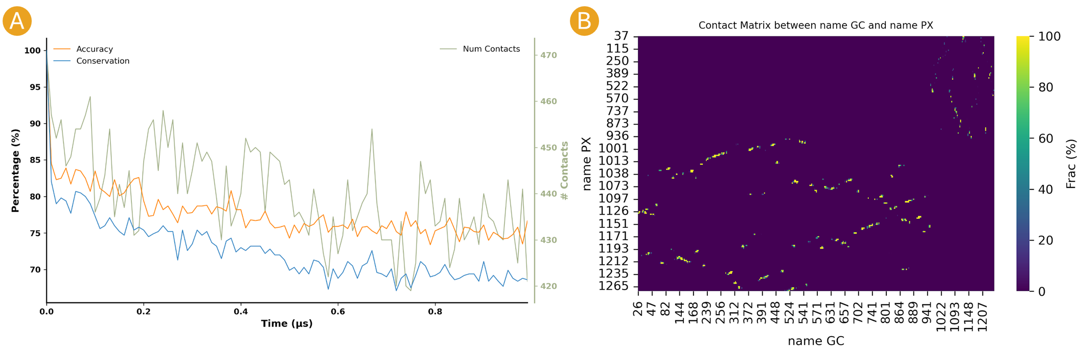
Figure 8. Intermolecular contact plots between the GC beads on the histone backbone and PX beads on the DNA phosphates of the NCP simulation. A) The native conservation plot displays the conservation of native contacts (blue), the accuracy of these contacts (orange), and the total number of contacts by frame (green) during the simulation. B) The contact map heatmap shows the average duration of the contacts within contact distance of one another during the simulation.

By clicking on the Contact Map button, a heatmap of the contact duration between residue pairs of the selections within contact distance of one another, expressed as a percentage of simulation time, is displayed (Figure 8B).

For further information on these plots and the .dat files, please see the Developers notes’ information about the Contacts tab.

Intramolecular contacts

To calculate intramolecular contacts, the choices must be in the same molecule.

For the NCP trajectory, let’s designate identical “name GC” selections on both boxes (Figure 9A).

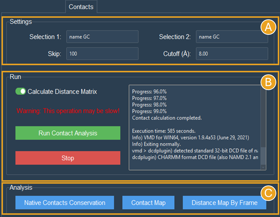
Figure 9. Contacts tab settings for intramolecular contacts analyses for the selections “name GC” of the NCP system. A) Settings to contact analysis. Two selections are needed, these selections can be in the same or different molecules. Here, both selections are identical and in the same molecule. The default numbers were set to speed up the calculation. B) Run contacts calculation. Since it was selected, a distance matrix will also be calculated. Calculation progress will be displayed and can be stopped at any time. C) When the calculations are done, buttons to make the plots will become active.

Let’s leave the cutoff distance at default value of 8.00 Å and use a 100-frame skip (reducing the 10.000-frame long trajectory to 100 frames) (Figure 9A).

Caution

Keep in mind that the calculation will take longer if the selections have many beads or atoms or if there are a high number of frames to be processed, so be patient.

Let’s select the Calculate Distance Matrix option (Figure 9B). The matrix here is symmetric as a result of the same number of GC beads on both selections. This symmetry is expected whenever the two interacting groups are of identical sizes, which is typically the case in intramolecular contact analyses.

Warning

Regardless of the selection, only GC (for proteins), PX (for DNA), or BFO (for lipids) beads are taken into consideration in the matrix to produce a concise distance matrix. This eliminates the need to calculate several distances between selections, hence it doesn’t create large files. For further information, please see the Developers notes’ information about the “Contacts” tab .

Click the Run Contact Analysis button (Figure 9B).

Tip

The VMD output area will display the progress of the calculation. The calculation can be stopped using the “Stop” button if something goes wrong.

Once the calculation is complete a new folder “Contacts” is generated in the working directory. To aid in the creation of the contact plots, the contact length, distance length, distbyframe, contacts, percentage, and timeline .dat files will be created.

Buttons for creating Native Contacts Conservation, Contact Map, and Distance Map By Frame plots will become active once the calculation is finished (Figure 9C).

By clicking on the Native Contacts Conservation button, a plot of the conservation of the initial frame contacts between the selections during the simulation can be obtained.

By clicking on the Contact Map button, a symmetric “name GC” by “name GC” heatmap is shown in an interactive window (Figure 10). In this window, a Colormap selector can be used to alter the color of the heatmap via a drop-down menu. A variety of Matplotlib colormaps (such as viridis, plasma, coolwarm, etc.) can be chosen to optimally highlight the contact pattern. Additionally, Matplotlib navigation (pan/zoom) is operable. Lastly, the plot can be exported at any resolution by using the “Save plot” option; just input the needed DPI number before saving.

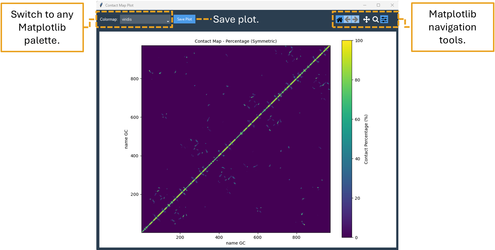
Figure 10. Contact Map plot window of the “name GC” by “name GC” matrix.

By clicking on the Distance Map by Frame button, the ‘Heat Map Viewer’ window will appear (Figure 11). A heatmap of the complete distance matrix between beads for every frame will be displayed. You can navigate among the frames or skip straight to a particular frame using a slider that is located over the plot. Similar to the “Contact map” panel, options for Matplotlib navigation and color palettes are accessible.

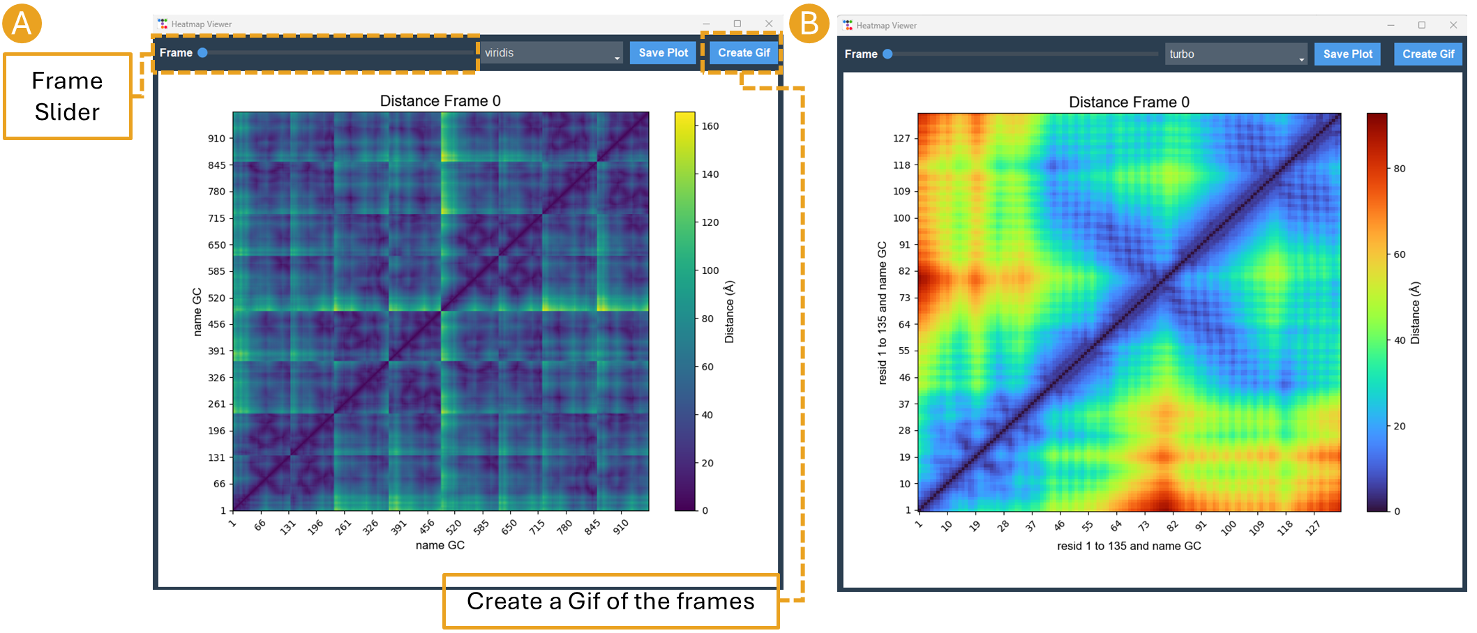
Figure 11. Heat map viewer. A) the heatmap for the “name GC” option, meaning the entire histone octamer, from the NCP simulation. B) To enhance visibility, we present an alternative selection utilizing a single histone.

Additionally, a Create GIF button (Figure 11) is provided to generate an animated GIF depicting the distance evolution throughout the experiment (Figure 12). Clicking “Create GIF” will generate a new folder titled “GIF” within the “Contacts” folder in the working directory.

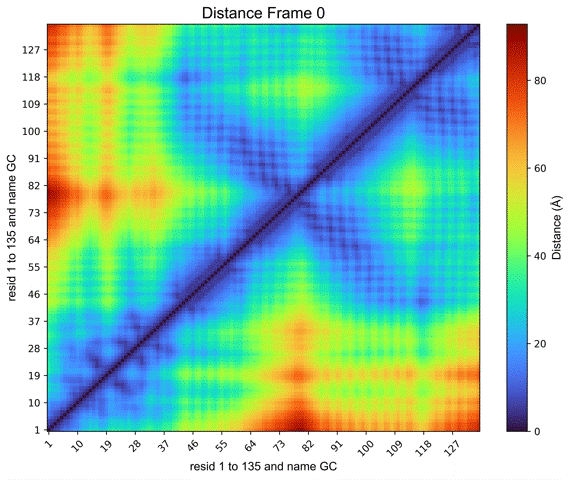
Figure 12. Animated GIF of 50 frames depicting one of the histones from the NCP simulation.

For further information on these plots and the .dat files, please see the Developers notes’ information about the “Contacts” tab.

Calculating Secondary Structure (SS)

Important

The SS Analysis tab uses the SIRAH Tools approach to categorize secondary structure elements (Helix, Extended Beta Sheet, or Coil), hence it is exclusively compatible with SIRAH MD simulations.

Here let’s select the SS Analysis tab. This tab allows performing secondary structure analysis throughout a SIRAH MD simulation using the methodology described in SIRAH Tools. See more details of the tab here.

For the NCP trajectory, let’s retain the default values for the “First” and “Last” fields (Figure 13A). The analysis will be conducted from the initial frame (1) to the final frame (-1). However, let’s modify the “Selection” field to the SIRAH macro “sirah_protein” and use a 10-frame skip in the trajectory (Figure 13A). This will speed up the calculations and reduce the number of frames from 10.000 to 1.000.

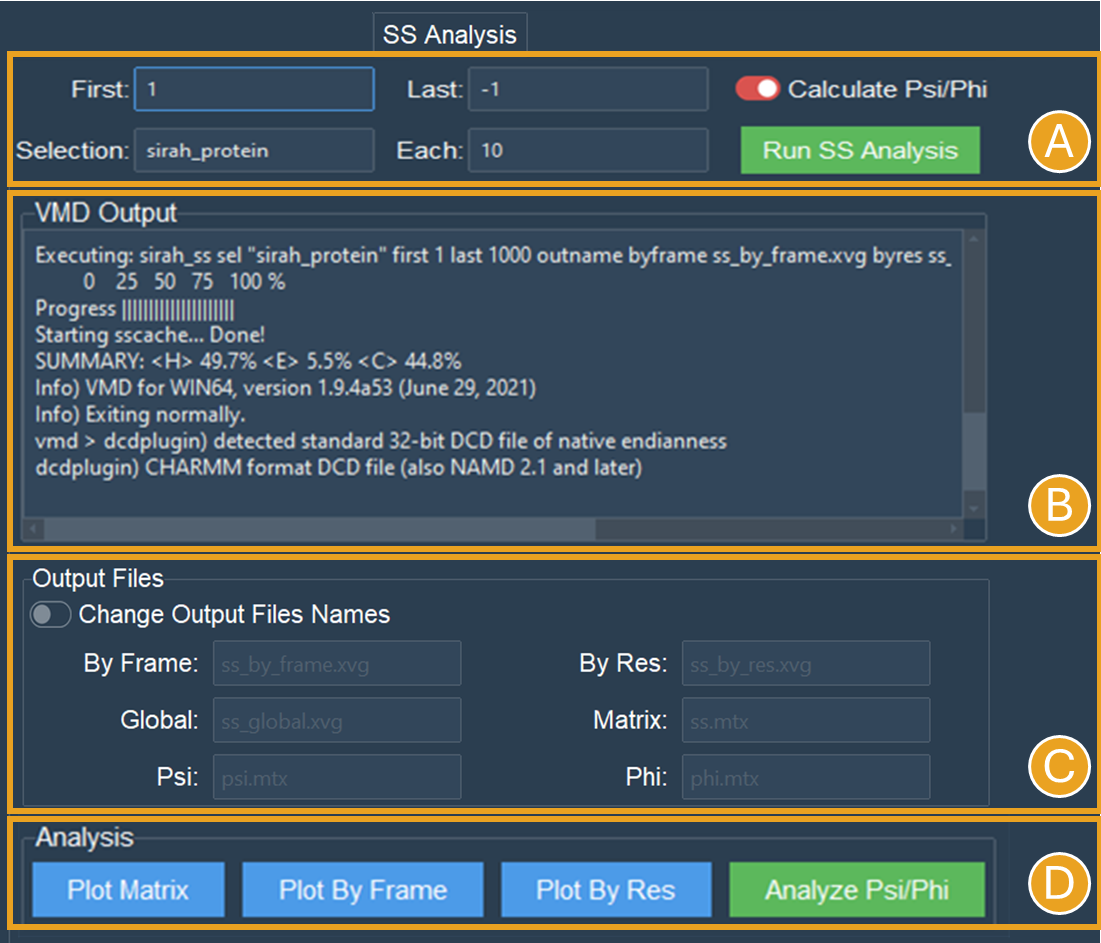
Figure 13. SS Analysis tab settings for secondary structure of the proteins in the NCP system. A) Settings to SS analysis. Here, the SS classification was calculated for the entire simulation using the default values and the sirah_protein macro. The Calculate Psi/Phi was also selected. B) The VMD output shows the progress of the calculation and the summary of SS the run. C) The names of the files created during the run. D) When the calculations are done, buttons to make the plots will become active.

Note

The interface allows for a selection; however, SS calculation is exclusively performed on protein structures. This selection, similar to those in other tabs, employs VMD syntax. Thus, for example, it allows for the calculation of information for particular chains within complicated protein systems.

Tip

Check out the SIRAH Tools tutorial to learn more about VMD and SIRAH macros and how to use them.

Let’s select the Calculate Psi/Phi option (Figure 13A). Selecting this option will compute the PSI/PHI angles during the secondary structure assignment and generate files suitable for plotting in a Ramachandran plot.

Click the Run SS Analysis button (Figure 13A). The VMD output area will exhibit the calculation progress, and a summary of the SS will be presented upon completion of the computation (Figure 13B). Leave the “Change Output File Names” unselected in the “Output Files” section (Figure 13C). Once the calculation is complete a new folder “ss_analysis” is generated in the working directory. To aid in the creation of the SS plots, the ss_by_frame.xvg, ss_by_res.xvg, ss_global.xvg, ss.mtx, phi.mtx, and psi.mtx files will be created. Buttons Plot Matrix, Plot by Frame, Plot by Res, and Analyze Psi/Phi will become active once the calculation is finished (Figure 13D).

Tip

The Analyse Psi/Phi option is always available in this tab. This indicates that prior angle calculations can be utilized at any moment, eliminating the need for repeated computations.

By clicking on the Plot Matrix button, a plot utilizing the ss.mtx file, displaying the alterations in secondary structure of each residue throughout the simulation will be generated (Figure 14A).

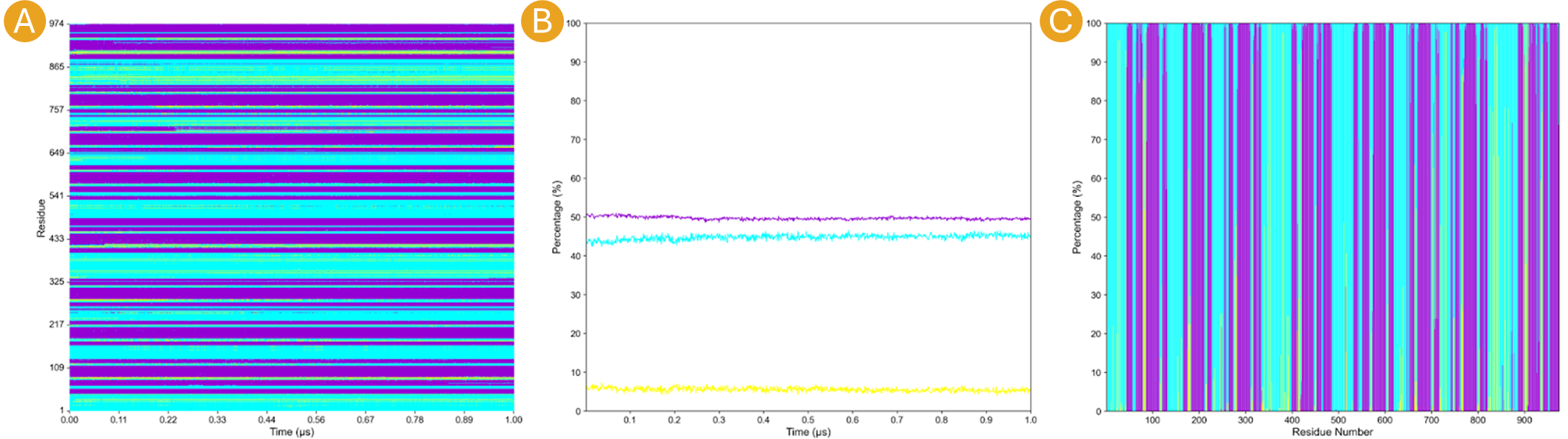
Figure 14. Outcomes of “Analysis” section from the SS Analysis tab where the secondary structural elements α-helix (H), extended β-sheet (E), and coil (C) are colored purple, yellow, and blue, respectively.

By clicking on the Plot By Frame button, a plot utilizing the ss_by_frame.xvg file, displaying the percentage changes of each secondary structure classification throughout the simulation will be generated (Figure 14B).

By clicking on the Plot By Res button, a plot utilizing the ss_by_res.xvg file, displaying the percentage of each secondary structure classification that each residue adopted throughout the simulation will be generated (Figure 14C).

By clicking on the Analyze Psi/Phi button, the Ramachandran Plot Visualization Tool window will appear (Figure 15). This interface allows for the loading of the psi.mtx and phi.mtx files via the Load PSI and Load PHI buttons, respectively (Figure 15A). A Ramachandran plot is automatically generated for the first frame (Figure 15B). You can also navigate among the frames using the frame slider or skip straight to a particular frame at the “Go to frame” option (Figure 15B).

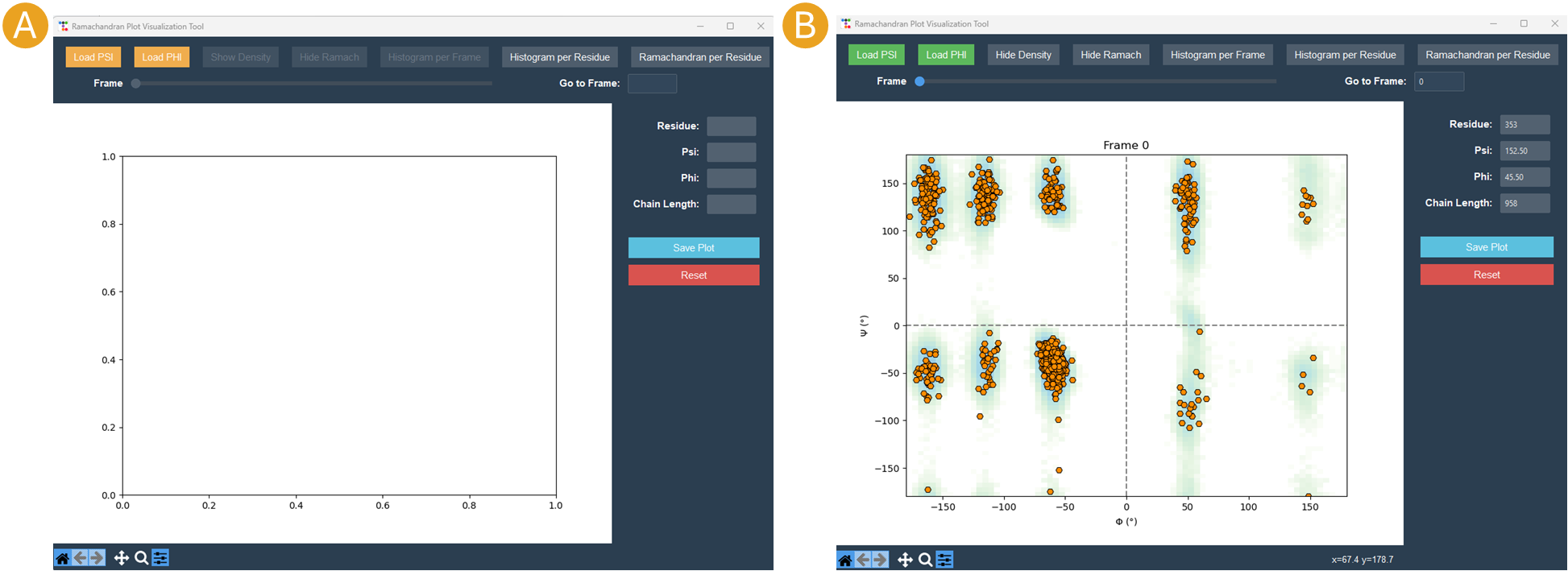
Figure 15. Ramachandran Plot Visualization Tool window. A) The window before loading the .mtx matrices. B) After loading the .mtx matrices. The Ramachandran plot of the Frame 0 is displayed with each residue as a point (orange). The overall density of the residues, using the position of the residues in the plot from all the frames, is also displayed (green areas).

Click on the “Show Density” button to display the density calculated for the entire matrix. Additionally, you can obtain particular information regarding the residue by hovering the mouse over a residue point (Figure 15B). Finally, select a frame and save the plot by clicking the Save Plot button.

Note

Depending on your screen’s resolution, the opened window may appear truncated; merely resize it to the appropriate dimensions.

For further information on the files and the Ramachandran Plot Visualization Tool, please see the Developers notes’ information about the SS Analysis tab .

Backmapping from CG to AA

Important

The Backmapping tab uses the SIRAH Tools approach, hence it is exclusively compatible with SIRAH MD simulations. Currently, backmapping libraries contain instructions for solute (proteins, DNA, metal ions, and glycans).

Here let’s select the Backmapping tab. This tab allows retrieving pseudo-atomistic information from the SIRAH CG model. The atomistic positions are built on a by-residue basis following the geometrical reconstruction (internal coordinates) to AA model. See more details of the tab here.

Caution

In the backmapping process, a structure minimization is performed using the AmberTools modules, therefore it is necessary to have configured the $AMBERHOME environment properly.

Optionally you can install AmberTools via conda:

conda install -c conda-forge ambertools=23

or more recently option:

conda install dacase::ambertools-dac=25

Remember to install it in the same Python environment created for SIRAH Tools GUI.

Note

SIRAH Tools GUI automatically detects if the $AMBERHOME environment is set in the system path (Figure 16A).

For the NCP trajectory, let’s retain the default values for the “First” and “Last” fields (Figure 16B). The analysis will be conducted from the initial frame (1) to the final frame (-1), meaning all frames will be used. However, let’s set a 5.000-frame skip in “Each” field to the trajectory (Figure 16B). This will bring the number of frames from 10.000 to 2.

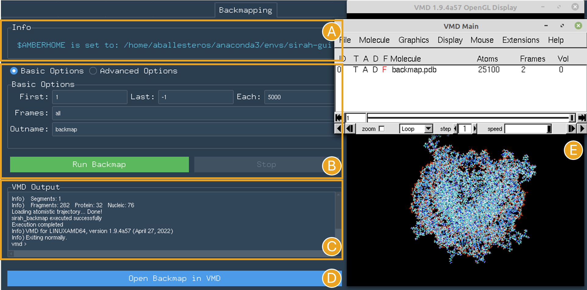
Figure 16. Backmapping tab settings for the NCP system when $AMBERHOME is set correctly. A) The $AMBERHOME environment was automatically detected and minimization using sander can be performed. B) In addition to applying a 5000-frame skip, all Basic Options and Advanced Options were retained at their default configurations within the SIRAH Tools. C) The VMD output shows the progress of the calculation. D) The Open Backmap in VMD button launches VMD with the backmap.pdb file. E) VMD windows with the backmap.pdb file.

Given that the $AMBERHOME environment is set up, minimization will be conducted with the default settings of the SIRAH Tools. Thus, click the Run Backmap button (Figure 16B). The VMD output area will exhibit the calculation progress (Figure 16C).

Upon completion of the calculation, a new folder titled “backmapping” is created in the working directory, containing a PDB or multi-PDB file entitled backmap.pdb. A Open Backmap in VMD will become activated (Figure 16D). This will open the generated PDB file in VMD (Figure 16E).

Warning

Always check both the original CG trajectory and the backmapping output to identify out-of-the-ordinary behavior and adjust arguments accordingly. Keep in mind that the minimized structures sometimes may differ from the CG trajectory due to the combination of all-atom minimization algorithms, number of cycles, cutoffs, etc.

Warning

In instances where AmberTools is unavailable, the nomin option, in the Advanced options section, can be used to disable the minimization step. Consequently, you can minimize backmapped outputs by utilizing other software/force fields outside of VMD. Keep in mind that hydrogen atoms won’t be added to the structures if the minimization step is skipped.

Let us examine a scenario in which the $AMBERHOME environment is not configured (Figure 17A).

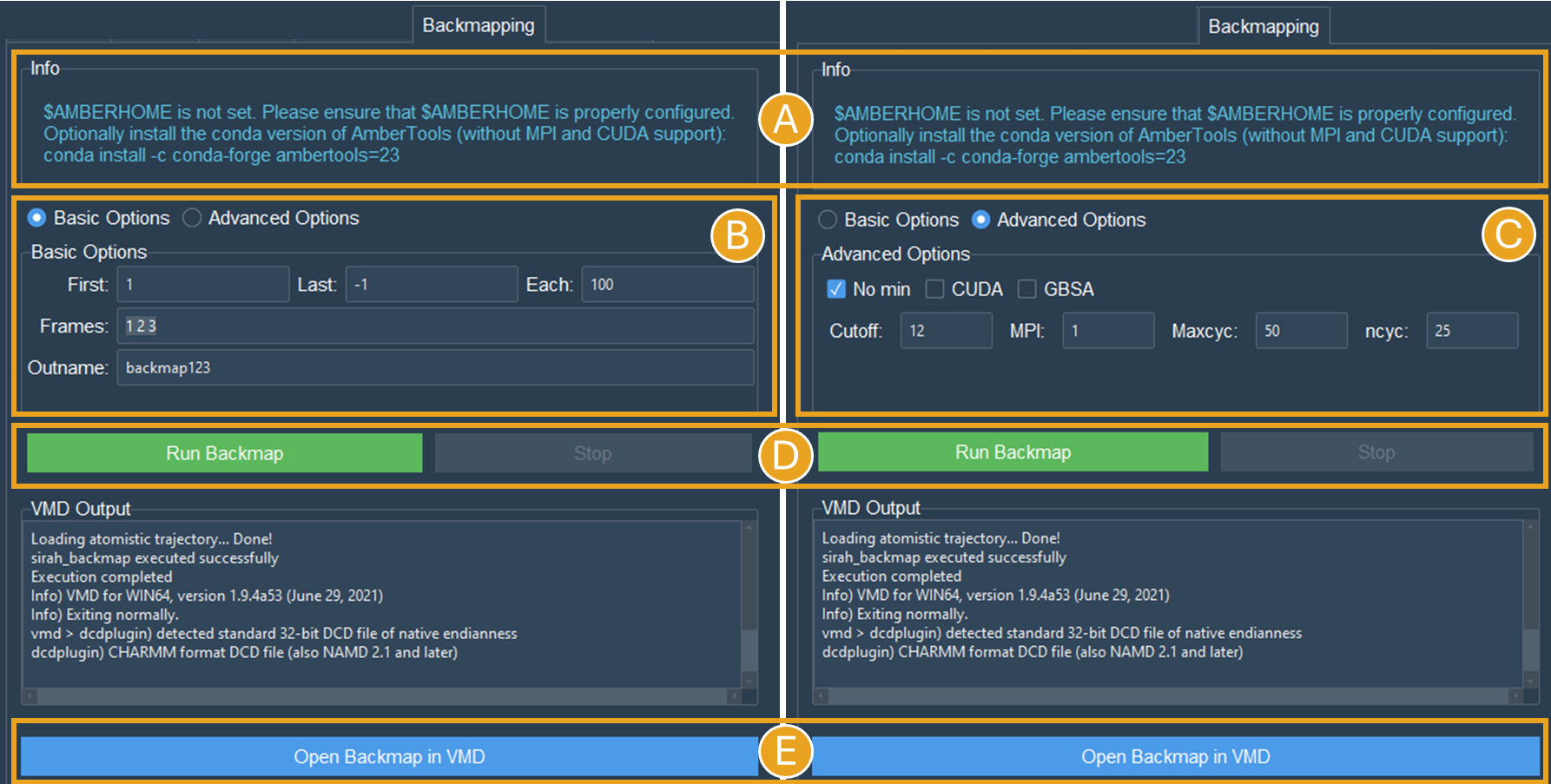
Figure 17. Backmapping tab settings for the NCP system when $AMBERHOME is not set correctly or not available. A) The $AMBERHOME environment was not detected and minimization using sander can not be performed. B) Configuration of the Basic Options via the Frames field. Since the “Frames” field has been established, the “First”, “Last”, and “Each” choices will be disregarded in the calculation. C) Configuration of the Advanced Options. Since the “nomin” option was selected, the other options, related to sander parameters will be disregarded in the calculation. D) Run Backmap button. E) The Open Backmap in VMD button launches VMD with the backmap.pdb file.

Rather than utilizing the complete trajectory, let us configure the Frames option (Figure 17B). This option requires a list of frames devoid of commas or dashes. Use “1 2 3” to obtain the backmapping of the initial three frames.

Note

The First/Last and Frames options are mutually exclusive. If Frames is specified, the First/Last and Each options are not used.

Let’s change the “Outname” from “backmap” to “backmap123” (Figure 17B).

Tip

Changing the “Outname” prevents the overwriting of previously backmapped frames.

To access the nomin option, use the Advanced Options radio button (Figure 17C). The Advanced Options includes additional settings, primarily associated with the minimization process. As we are utilizing the “nomin” option, let us keep the other options as they are.

Click the Run Backmap button (Figure 17D) and examine the backmap123.pdb file in PDB by selecting Open Backmap in VMD (Figure 17E).

For further information on this tab options, please see the Developers notes’ information about the Backmapping .

Developers notes

Here, we provide further technical information regarding each SIRAH Tools GUI tab as well as details on identified issues and limitations.

General Information

This section offers information that is identical or analogous to all SIRAH Tools GUI tabs:

• The SIRAH Tools GUI works with VMD in text mode; therefore, it can be used on any system that can be loaded in VMD.

• The GUI automatically detects if VMD is set in the system path, this is essential for the correct operation of SIRAH Tools GUI. If VMD is not set up correctly, a warning will be displayed and the tabs will be disabled.

• SIRAH Tools GUI uses VMD syntax selections (e.g. name, resname, resid, etc.) or VMD/SIRAH macros in all selection boxes. Check out the SIRAH Tools tutorial to learn more about VMD and SIRAH macros and how to use them.

• Use caution regarding excessively big or heavy trajectories. To minimize computer memory usage, SIRAH Tools GUI terminates VMD after completing an analysis on a tab. This indicates that if the analysis requires repetition or the user navigates to a different tab, the trajectory file will be reloaded in both scenarios. Therefore, we advise utilizing the skip frame options in the tabs (when available) or reducing the system size (for example, by eliminating solvent molecules) to decrease the loading time.

• The VMD output area presents details regarding the VMD execution alongside the terminal window in which the SIRAH Tools GUI was initiated. Consequently, any issue or malfunction within SIRAH Tools GUI will show up in these locations.

• Any external plotting software or script should be able to use the files in text format generated from the conducted analysis.

• The plots produced by the SIRAH Tools GUI, which feature simulation time as an axis, are on the microsecond timeframe to align with the expected simulation duration of microseconds for the SIRAH force field.

• Complex systems that contain an excessive number of components might lead to plots that are densely packed.

• Depending on your screen’s resolution, the GUI window may appear truncated; merely resize it to the appropriate dimensions.

• The SS Analysis and Backmapping tabs use the SIRAH Tools approach, hence it is exclusively compatible with SIRAH MD simulations.

Load Files

The Load Files tab allows loading AMBER, GROMACS, and NAMD simulation topologies and trajectories compatible with SIRAH force field MD simulations (Figure 18).

Note

The SIRAH Tools GUI works with VMD in text mode; therefore, it can be used on any system that can be loaded in VMD.

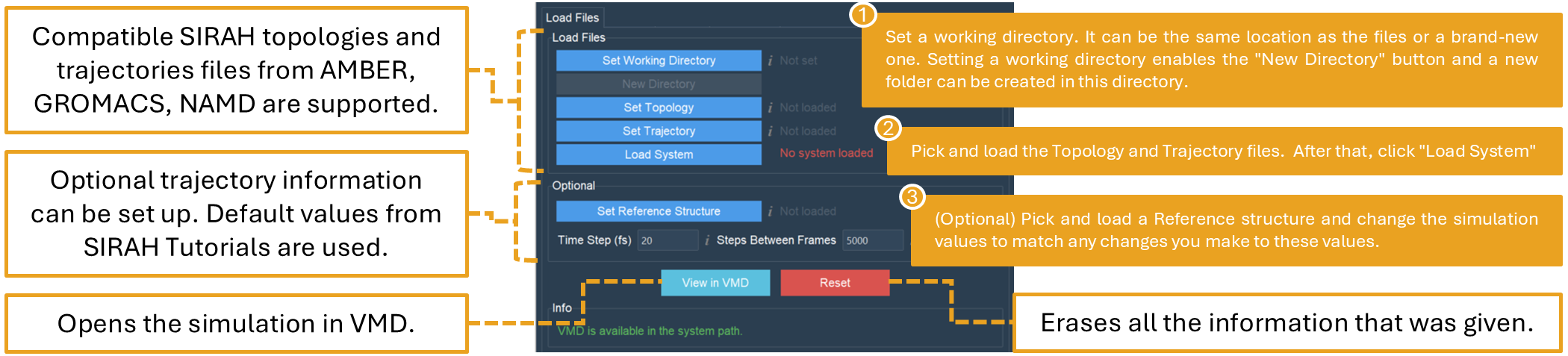
Figure 18. The Load Files tab. Setting up any subsequent analysis with the SIRAH Tools GUI begins with the “Load Files” tab.

Warning

Windows may not support AMBER trajectories in NetCDF format (limited by VMD).

Optionally, the user can load a reference structure (pdb or gro format are supported) to be used for RMSD and RMSF calculations. In addition, the time step and step between frames boxes are set to the default values used in the SIRAH tutorials. If these values have been changed, users must set them to the right values used in their simulation to make sure the analyses and plots are performed correctly.

Note

The GUI automatically detects if VMD is set in the system path, this is essential for the correct operation of SIRAH Tools GUI. If VMD is not set up correctly, a warning will be displayed and the tabs will be disabled.

Caution

Use caution regarding excessively big or heavy trajectories. To minimize computer memory usage, SIRAH Tools GUI terminates VMD after completing an analysis on a tab. This indicates that if the analysis requires repetition or the user navigates to a different tab, the trajectory file will be reloaded in both scenarios. Therefore, we advise utilizing the skip frame options in the tabs (when available) or reducing the system size (for example, by eliminating solvent molecules) to decrease the loading time.

Analysis

The Analysis tab allows several types of MD simulation analysis (Figure 19). Basic (RMSD, RMSF, and Radius of Gyration (RGYR) and advanced analyses (SASA, measuring the distances between two beads, and Radial Distribution Functions (RDF) are available.

The number of selection entries that the user must provide is where basic and advanced analysis diverge. While up to two entries can be made for advanced analysis, only one selection entry is required for basic analysis. VMD syntax selections (e.g. name, resname, resid, etc.) or VMD/SIRAH macros must be entered in all selection boxes.

Tip

Check out the SIRAH Tools tutorial to learn more about VMD and SIRAH macros and how to use them.

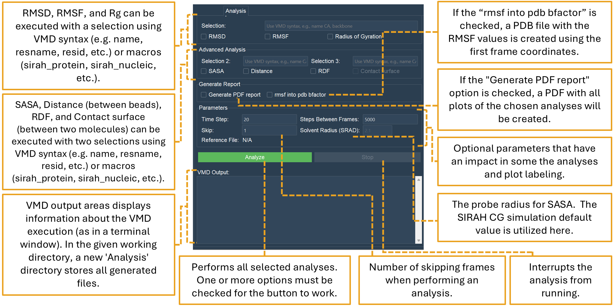
Figure 19. The “Analysis” tab performs and plots common MD analysis routines.

Note

The “Analyze” button will only be enabled if one or more options are selected in either the Basic Analysis or Advanced Analysis sections, but you are not required to check every checkbox.

The following information is used to calculate Basic Analysis options in SIRAH Tools GUI:

• RMSD: the VMD measure command is used to calculate RMSD (see VMD measure ). Prior to RMSD calculation, each frame of the trajectory will be superimposed to the first frame or the reference structure based on the selected syntax. Thus, all beads or atoms of the selection will be rotated and translated to fit a structure (first or reference) to minimize RMSD. There isn’t currently a nofit option.

• RMSF: the VMD measure command is used to calculate RMSF (see VMD measure ). This command returns the root mean square position fluctuation for each selected bead or atom in the selected frames. Prior to RMSF calculation, each frame of the trajectory will be superimposed to the first frame or the reference structure based on the selected syntax. Thus, all beads or atoms of the selection will be rotated and translated to fit a structure (first or reference). There isn’t currently a nofit option. The output file is provided based on bead or atom numbers.

• RGYR: the VMD measure command is used to calculate RGYR (see VMD measure ). This command returns the radius of gyration of atoms in the selection. The calculation is done for all frames.

Important

It is necessary to fill out both selections in the Advanced Analysis.

The following information is used to calculate Advanced Analysis options in SIRAH Tools GUI:

• SASA: the VMD measure command is used to calculate SASA (see VMD measure). So, a selection in VMD syntax (e.g. name, resname, resid, etc.) or VMD/SIRAH macro is needed to calculate SASA (Selection2). There is, however, a restrictedsel flag in the command as well, implemented here as the second selection (Selection3). This flag limits the calculation to the solvent-accessible points close to this restricted region. This keeps protein voids or pockets inside the protein from affecting the surface area values. For the SIRAH Tools GUI, the restrictedsel flag is not used if Selection2 and Selection3 are the same. If they are different, however, Selection3 will be used as the restrictedsel flag. Refer to the Basic Analyses VMD tutorials SASA section .

• RDF: the VMD measure command is used to calculate Radial Distribution Function (RDF) (see VMD measure). Given that typical RDF is calculated between two items, both Selection2 and Selection3 must be defined and have to reference the same molecule. However, Selections 2 and 3 may be the same or dissimilar. Very complex distribution functions can be calculated thanks to the strength of VMD’s selection language syntax. In addition, here, the maximum radius to calculate RDF is set to 12 Å.

• Distance: to determine the distance between the selections, SIRAH Tools GUI computes their center of mass using the VMD measure command (see VMD measure). Therefore, only two distinct selections—for example, two distinct atoms or beads, two distinct residues, two distinct molecules, etc.—can be used to calculate the “Distance” option. If they are identical molecules, residues, beads, or atoms, meaning using the same selection in both selection boxes, will result in a zero value to all frames.

The “Generate Report” section also offers two options: if the “Generate PDF report” option is chosen, a PDF with all plots of the chosen analyses will be created. If the “rmsf into pdb bfactor” is checked, a PDB file with the RMSF values in the Beta factor column is created using the first frame coordinates.

There are further options in the “Parameters” section. While the “Skip” option relates to skipping frames when performing an analysis, the “Time Step” and “Step Between Frames”, which are retrieved from the “Load Files” page, can also be changed here. These parameters should be entered properly since they will have an impact on the plot labels.

Note

If different values of “Time step” and “Step between frames” have been applied in the MD simulation, users must set them to the appropriate values used in their simulation to make sure the analyses and plots are performed correctly.

The reference file is yet another bit of data that may be obtained from “Load Files”. The RMSD and RMSF analyses will be performed using the reference file, if one was loaded.

Additionally, it is possible to set the “Solvent Radius (SRAD)” for SASA calculations. SRAD is the probe radius utilized for the SASA analysis in VMD. The default value chosen here (2.1 Å) is the one used in CG simulations in SIRAH.

Tip

The VMD output area displays information about the VMD execution (as in a terminal window). Thus, any problem or error within the VMD will appear here.

In the given working directory, a new “Analysis” directory will store all generated files, plots, reports, and PDB files.

Note

The name of the files consists of a ‘root’ according to the analysis concatenated with the selection. The way that the files are named facilitates the analysis of various selections. New files are created by different selections, whereas files are rewritten over if the same selection is made again. Nevertheless, a pop-up box will question if the user wants to rewrite the files.

Contacts

The Contacts tab allows the analysis of contacts between two selections using a cutoff distance as a criterion (Figure 20). It produces native contact data, contacts and distance maps. Intermolecular or intramolecular contacts can be calculated depending on the selection. In addition, the “Calculate Distance Matrix” option allows to compute a distance matrix of each pair of beads for each frame of the simulation.

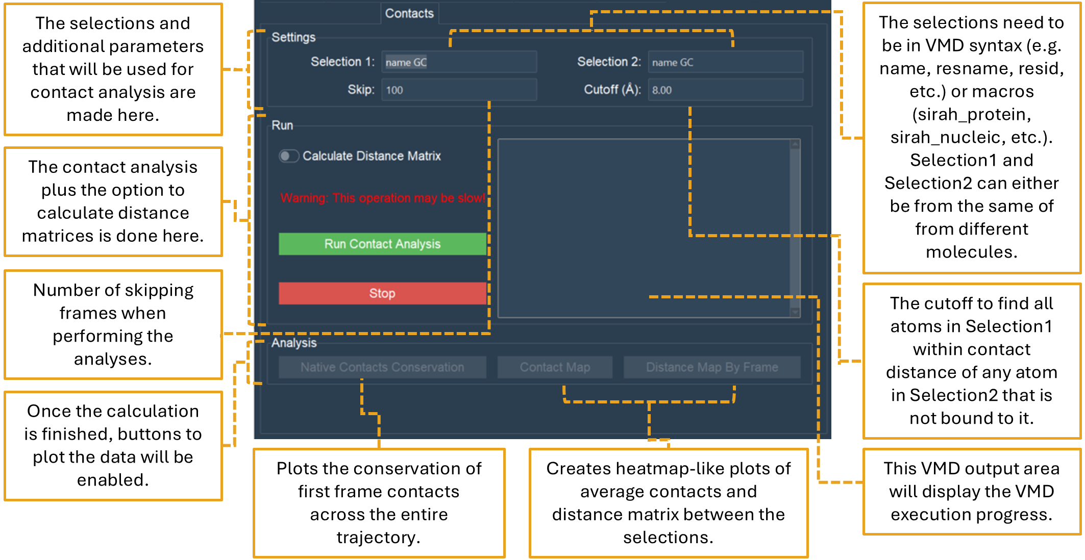
Figure 20. The “Contacts” tab performs and plots different contact analysis routines.

Note

If the selection contains many atoms or if it has too many frames, the distance matrix calculation can be slow and demanding.

In the “Settings” section, two selections in VMD syntax are needed. When Selection1 and Selection2 are in the same molecule, intramolecular contacts are calculated. When Selection1 and Selection2 are in different molecules, intermolecular contacts are calculated. The default distance cutoff value to determine a contact is 8.00 Å, generally used to analyze SIRAH simulations. The “Skip” option will decrease the number of frames of the trajectory to be processed by the value chosen by the user. In order to improve the calculation for longer trajectories, the default value is 100.

In the “Run” section, a “Calculate Distance Matrix” option can be found. If this option is enabled, a distance matrix of the selections will be calculated for every frame of the trajectory. Depending on the number of the frames this calculation can be quite slow.

Warning

Regardless of the selection, only GC (for proteins), PX (for DNA), or BFO (for lipids) beads are taken into consideration in the matrix to produce a concise distance matrix. This eliminates the need to calculate several distances between selections, hence it doesn’t create large files.

Tip

The VMD output area will display the progress of the calculation. The calculation can be stopped using the “Stop” button if something goes wrong.

The “Analysis” section will be enabled once the calculation is finished. Three buttons will be available:

1. Native Contacts Conservation that plots the conservation of the first frame contacts between the selections during the simulation. The native contact conservation plot is a line graph with the simulation time on the X-axis and the percentage of contacts on the Y-axis. A secondary Y-axis representing the number of contacts found is also illustrated. This graph depicts three elements:

• The percentage of contact conservation during the simulation (blue line), utilizing the initial frame as the reference point. This approach involves dividing the quantity of conserved contacts identified in a frame by the quantity of conserved contacts identified in the reference frame;

• The percentage of contact accuracy during the simulation (orange line). This calculation involves dividing the quantity of conserved contacts identified in a frame by the entire quantity of contacts present in that same frame;

• The number of contacts that yields the overall amount of contacts for each frame (green line). The defined cutoff distance is used to determine all beads or atoms that are within contact distance of the selections.

2. Contact Map that plots a heatmap with the total interaction time, in simulation time percentage, between the residues of the selections during the simulation.

• The contact map heatmap utilizes data from all contacts within the specified cutoff to compute an average residue-by-residue persistence duration of the contacts in the trajectory. Based on the selection, several beads or atoms of a single residue may interact with numerous beads or atoms of another residue; therefore, to eliminate repetition, only the interacting pair with the highest frame count is utilized in the plot. However, a file with the information of all the interacting pairs is created to be used by the user. In addition, a standard Matplotlib navigation (pan/zoom) is presented, showcasing various accessible color combinations.

3. Distance Map by Frame that plots the distance between the selections as a heatmap for each frame, independent of the cutoff distance. In this analysis, users can move through the frames, save the plot, and make a gif in the pop-up window that appears.

• The vecdist command of VMD is used to calculate the distance for the distance matrix, where the two vectors represent the coordinates of two selections. It is recommended to utilize selections that yield a singular bead or atom per residue for this plot. When dealing with selections that included several beads or atoms per residue, the computation performed for each frame led to prolonged calculations, elevated memory consumption, and huge files. Therefore, if a selection has many beads or atoms per residue (such as in the macro sirah_protein or protein), the TCL script (/TCL/contacts_distance.tcl) will automatically select one backbone bead (GC, PX or BFO) or atom (CA, P) for the selection. This decision enhances visualization, accelerates computation, and eliminates the necessity for generating large files.

Note

To generate an animated GIF of the distance heatmap, select the “Create GIF” button in the Matplotlib window. You will be required to input the starting and ending frame numbers, the DPI for each frame image, and indicate whether to delete the individual frame images after the GIF has been created. The tool will produce all needed images and compile them into a GIF within the new ‘Contacts/GIF’ folder in your working directory. If you opt to retain the single-frame files, they remain in that directory alongside to the GIF.

Once the calculation is complete a new folder “Contacts” is generated in the working directory. To aid in the creation of the contact plots, the “contact length”, “distance length”, “distbyframe”, “contacts”, “timeline’, and “percentage” .dat files will be created. A description of the content of each file is provided below:

• The contact length and distance length files contain the dimensions of the matrix and the information on the selections for the contact and distance heatmaps.

• The contacts file contains a general summary of the native contact conservation, accuracy, and total number of contacts from the simulation.

• The timeline file summarizes the conservation of native contacts, accuracy, and the total number of contacts for each frame, categorizing them as either native or non-native within the specified cutoff for each frame.

• The distbyframe file contains a distance matrix for each analyzed frame with the distance between every pair of selections.

• The percentage file contains the information on the percentage of duration of all contacts within the defined cutoff from the simulation. To ensure that all contacts are recorded in the file, the information is provided utilizing the residues and the beads (atoms) for each contacting pair.

Tip

Any external plotting software or script should be able to use these .dat files.

SS Analysis

Important

The SS Analysis tab uses the SIRAH Tools approach to categorize secondary structure elements (Helix, Extended Beta Sheet, or Coil), hence it is exclusively compatible with SIRAH MD simulations.

The SS Analysis tab allows the classification and analysis of secondary structure elements using the methodology described in SIRAH Tools (Figure 21). It classifies proteins in a SIRAH MD simulation into α-helix (H), extended β-sheet (B), or Coil (C). Additionally, it computes PSI/PHI angles that can be illustrated in a Ramachandran plot.

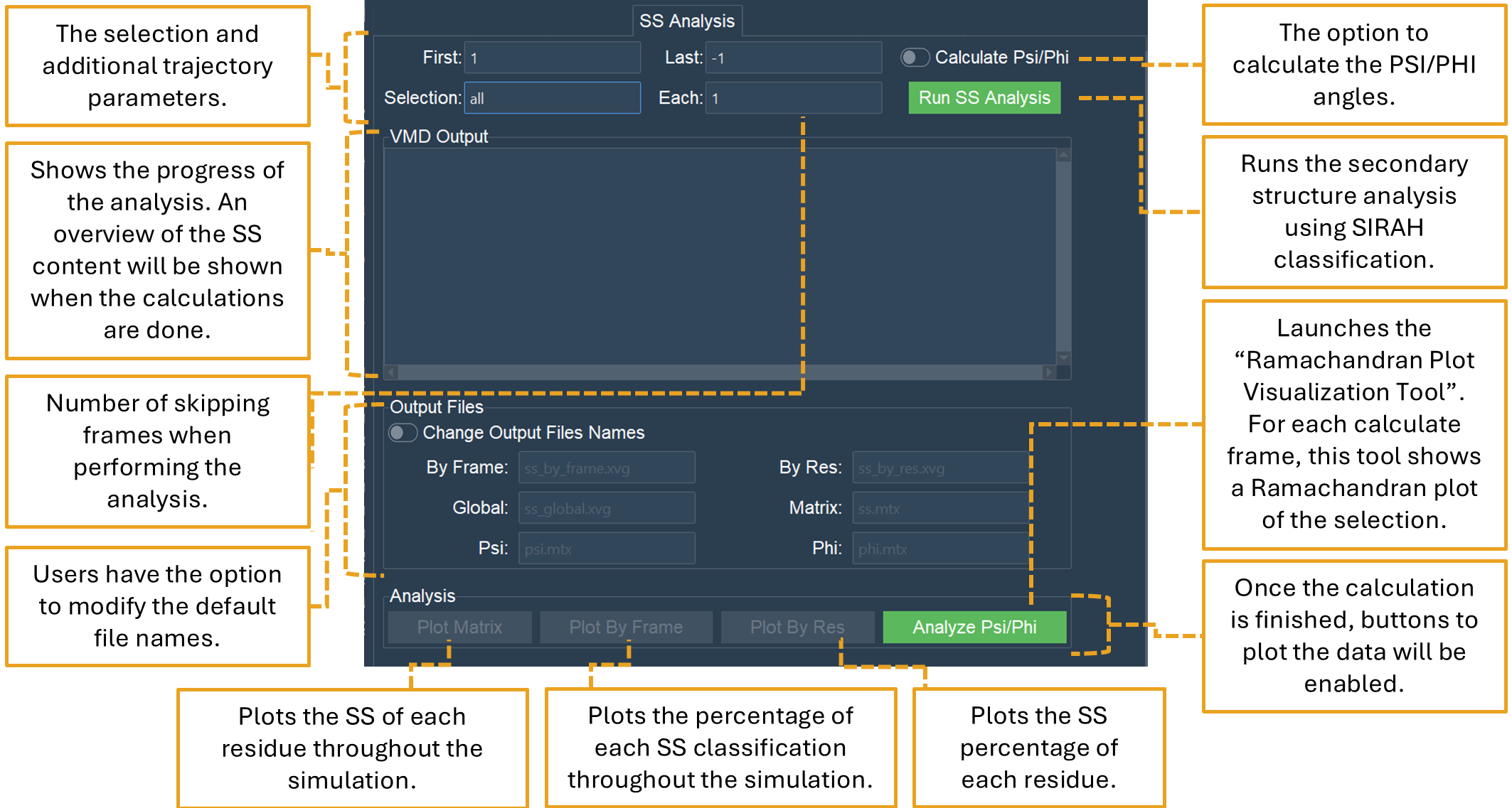
Figure 21. The SS Analysis tab performs and plots SS content for SIRAH MD simulations.

Users can select a frame interval for calculating the secondary structure from the trajectory. By default, the computation is performed from the initial frame (1) to the final frame (-1) of the trajectory. Nonetheless, any numerical interval may be utilized. The “Each” option is similar to the “Skip” option in other tabs and will decrease the number of frames of the trajectory to be processed by the value chosen by the user. The default value is 1, hence no frame skipping occurs.

The interface also enables a selection for the calculation; by default, the entire system is selected. This selection, similar to the other tabs, employs VMD syntax or SIRAH Tools Macros.

The CG backbone torsional angles PSI and PHI can be computed together with the secondary structure from the trajectory by activating the “Calculate Psi/Phi” option. This will generate two matrices and files, one for PSI (psi.mtx) and one for PHI (phi.mtx), including the angle values of each residue across all frames within the selected interval. The generated PSI and PHI files are suitable for a Ramachandran plot.

Note

The CG PSI/PHI angles are calculated using the transformations specified in Machado et al to facilitate comparison with canonical secondary structure elements in the atomistic Ramachandran plot. This ensures that the torsional energy landscape is represented in the same AA geometrical space. For additional details, check Machado et al.

In the Output Files section, the name of each file to be generated can be modified. This reduces the possibility of overwriting previously produced files.

The Run SS Analysis button will examine all the established parameters and execute the SS content analysis.

The VMD output area will display the progress of the calculation. Upon completion of the calculation, the “ss_analysis” folder is created in the working directory, containing the files: ss_by_frame.xvg, ss_by_res.xvg, ss_global.xvg, ss.mtx, and if the Phi/Psi analysis option was enabled, the files phi.mtx and psi.mtx are additionally produced.

The “Analysis” section buttons will be enabled once the files are created. Four buttons will be available:

1. Plot matrix that plots the ss.mtx. The ss.mtx file encompasses a matrix that illustrates the variation in the SS of each residue throughout the simulation. This plot displays three colors according to the SS classification: purple for H, yellow for B, and cyan for C.

2. Plot by frame that plots the by_frame.mtx. The by_frame.mtx file encompasses the percentage changes of each SS content throughout the simulation. This plot is a line plot, displaying three colors according to the SS classification: purple for H, yellow for B, and cyan for C.

3. Plot by Res that plots the ss_by_res.mtx`. The ss_by_res.mtx file encompasses the percentage of each SS classification that each residue adopted throughout the simulation. This plot will display three colors according to the SS classification: purple for H, yellow for B, and cyan for C.

“Analyze Psi/Phi” launches the “Ramachandran Plot Visualization Tool” interface (Figure 22). This interface allows for the loading of the psi.mtx and phi.mtx files via the “Load PSI” and “Load PHI” buttons, respectively. A Ramachandran plot is automatically generated to all chosen frames and can be iterated by using the “Frame” slider or “Go to frame” option.

Tip

The “Analyse Psi/Phi” option is always available in this tab. This indicates that prior angle calculations can be utilized at any moment, eliminating the need for repeated computations.

Note

The ss_global.xvg file is not plotted since it only shows the overall percentages and standard deviation of H, E, and C of the entire simulation.

The “Ramachandran Plot Visualization Tool” allows for the loading of the psi.mtx and phi.mtx files via the “Load PSI” and “Load PHI” buttons, respectively (Figure 22A). A Ramachandran plot is automatically generated for the first frame (Figure 22B), however plots are created for all frames. The “Frame” slider or the “Go to frame” option can help navigate among the frames. The “Show Density” button displays the density computed for the full matrix, but the “Hide Ramach” option conceals the residue points in the plot. Histogram buttons, “Histogram per Frame” and “Histogram per Residue”, allow the creation of histograms for each frame or for a specific residue, respectively. Additionally, the “Ramachandran per residue’ button displays the angles of a specific residue in the Ramachandran geometrical space.

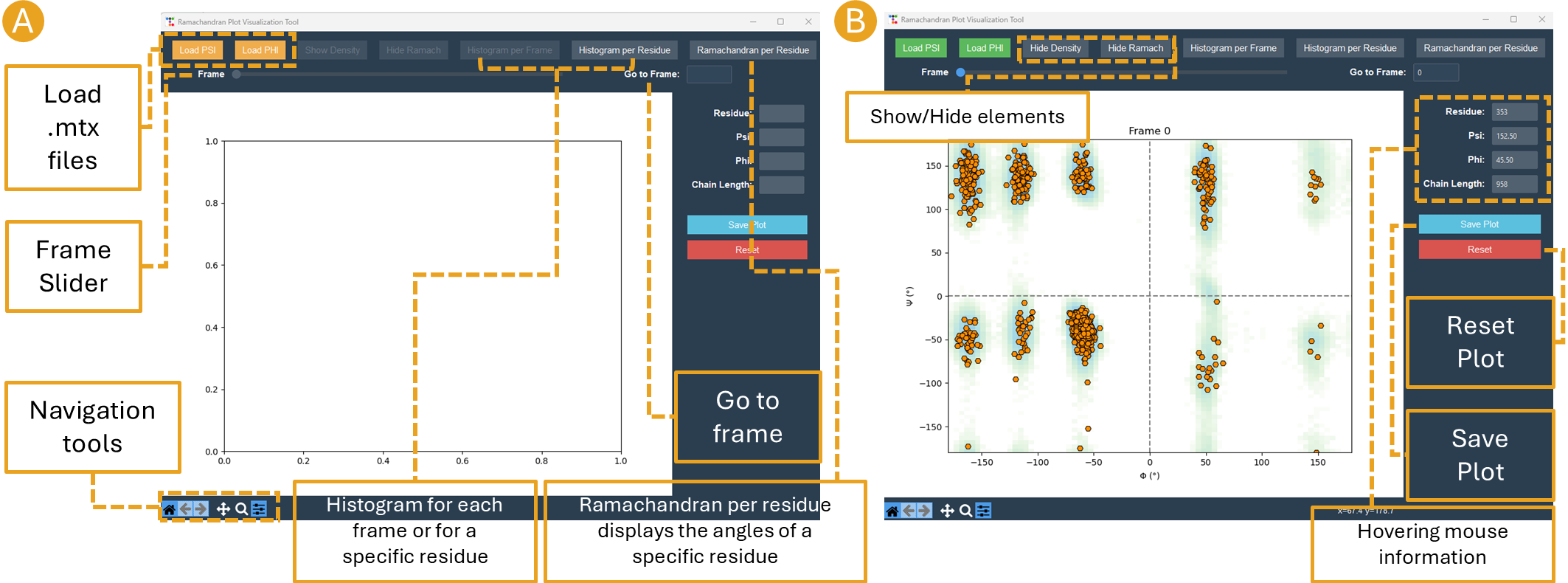
Figure 22. Ramachandran Plot Visualization Tool window. A) The window before loading the .mtx matrices. B) After loading the .mtx matrices. The Ramachandran plot of the Frame 0 is displayed with each residue as a point (orange). The overall density of the residues, using the position of the residues in the plot from all the frames, is also displayed (green areas).

Positioning the mouse over a residue point reveals specific information about the residue on the right side of the “Ramachandran Plot Visualization Tool”. Also on the right side, “Save Plot” and “Reset” buttons are found to save the Ramachandran plot for a frame and return the tool to its initial state, respectively.

Note

Depending on your screen’s resolution, the opened window may appear truncated; merely resize it to the appropriate dimensions.

Backmapping

Important

The Backmapping tab uses the SIRAH Tools approach, hence it is exclusively compatible with SIRAH MD simulations. Currently, backmapping libraries contain instructions for solute (proteins, DNA, metal ions, and glycans).

The Backmapping tab allows retrieving pseudo-atomistic information from the SIRAH CG model (Figure 23). The atomistic positions are built on a by-residue basis following the geometrical reconstruction (internal coordinates) to AA model. Bond distances and angles are derived from rough organic chemistry considerations stored in backmapping libraries. Next, the structures from the initial stage are protonated and minimized with the atomistic force field ff14SB within the tleap module of AmberTools. A PDB or multi-PDB file entitled backmap.pdb will be created at the end of the calculation.

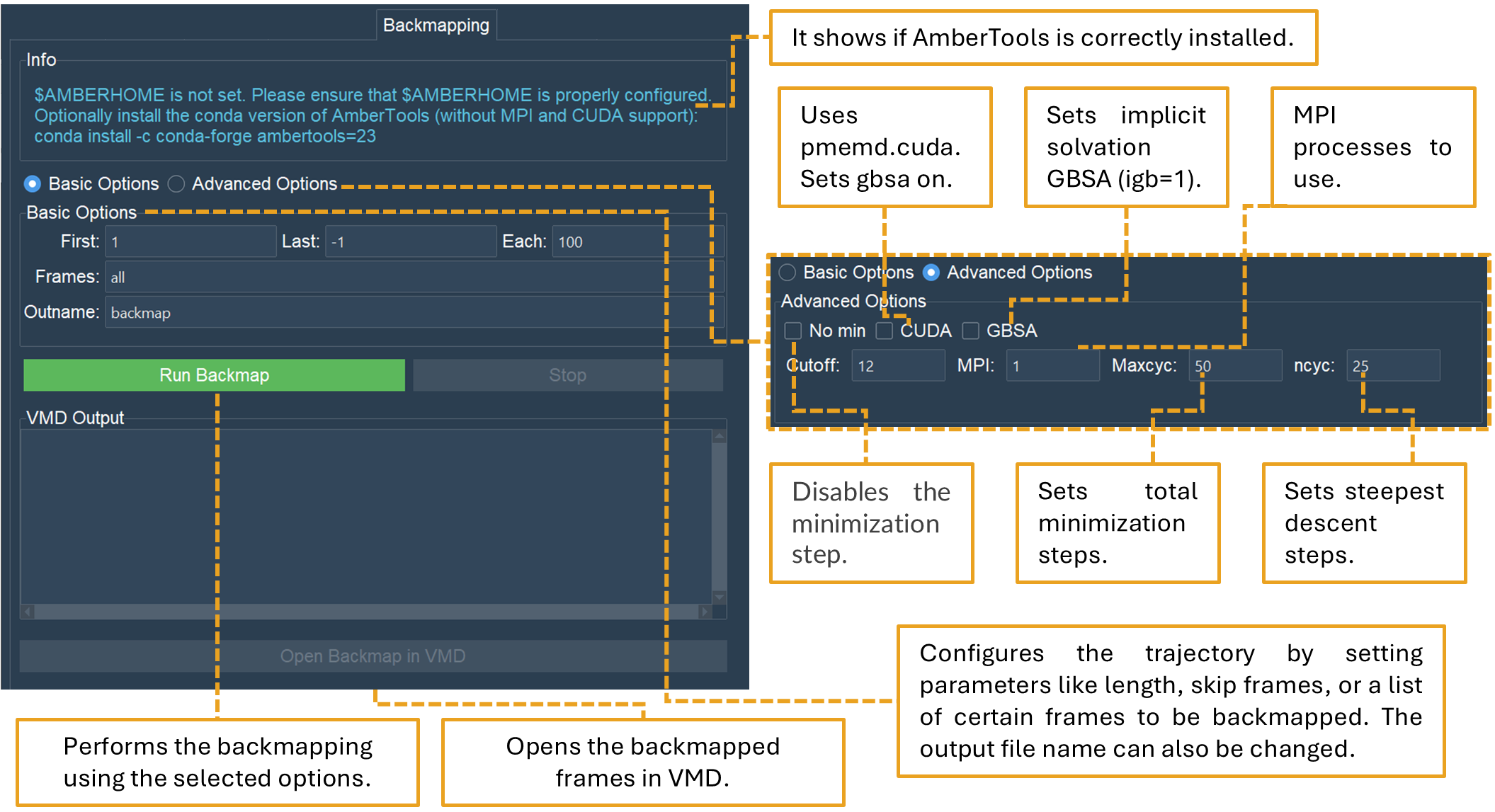
Figure 23. The “Backmapping” tab performs backmapping for SIRAH MD simulations.

Caution

SIRAH Tools GUI automatically detects if the $AMBERHOME environment is set in the system path (Figure 23). If the $AMBERHOME environment is not correctly configured, the structure minimization in the backmapping process cannot be executed, as it relies on AmberTools modules. The backmapping can still be done using the “nomin” option in the Advances Options section (Figure 23). Consequently, these structures can be minimized by utilizing other software/force fields outside of VMD.

Note

Keep in mind that hydrogen atoms won’t be added to the structures if the minimization step is skipped.

Tip

Optionally you can install AmberTools via conda (without MPI and CUDA support):

conda install -c conda-forge ambertools=23

or more recently option:

conda install dacase::ambertools-dac=25

Remember to install it in the same Python environment created for SIRAH Tools GUI. This should be enough to configure AmberTools for compatibility with the SIRAH Tools GUI.

In the Basic Options section, users can select a frame interval for backmapping structures from the trajectory. By default, the computation is performed from the initial frame (1) to the final frame (-1) of the trajectory. Nonetheless, any numerical interval may be utilized. The “Each” option is similar to the “Skip” option in other tabs and will decrease the number of frames of the trajectory to be processed by the value chosen by the user. The default value is 100, hence the number of trajectory frames will be divided by 100. However, any numerical value may be used.

Caution

Keep in mind that the calculation will take longer if there are too many elements to backmap or if there are a high number of frames to be processed, so be patient.

A list of specific frames can also be used in the “Frames” option. The list of frames needs to be devoid of commas or dashes, like “1 2 3”.

Note

The First/Last and Frames options are mutually exclusive. If Frames is specified, the First/Last and Each options are not used.

In the Outname option, the name of the output file to be generated can be modified. The default name is “backmap”.

Tip

Changing the “Outname” prevents the overwriting of previously backmapped frames.

In Advanced Options section, you could set options related to the minimization of the backmapped frames:

• nomin: Option to avoid minimizing the system;

• mpi: MPI processes to use during minimization, default 1;

• CUDA: Flag to use pmemd.cuda, sets GBSA on, cutoff to 999 and no MPI;

• GBSA: Flag to use implicit solvation GBSA (igb=1), default off (igb=0);

• cutoff: Set cut-off value (in angstroms) for non-bonded interactions, default 12;

• maxcyc: Set total number of minimization steps, default 150;

• ncyc: Set the initial number of steepest descent steps, default 100.

Note

In most cases, the default parameters of 100 steps of steepest descent (ncyc) and 50 steps of conjugate gradient (total of 150 maxcyc steps) in vacuum conditions are sufficient to produce a correct result. Depending on the system, users can increase or decrease these values to have better results.

Warning

Always check both the original CG trajectory and the backmapping output to identify out-of-the-ordinary behavior and adjust arguments accordingly. Keep in mind that the minimized structures sometimes may differ from the CG trajectory due to the combination of all-atom minimization algorithms, number of cycles, cutoffs, etc.

The “Run Backmap” button will examine all the established parameters and execute the backmapping. The calculation can be stopped using the “Stop” button if something goes wrong.

The VMD output area will display the progress of the calculation. Upon completion of the calculation, the “Backmapping” folder is created in the working directory, containing the backmap.pdb file. If all went well, the “Open Backmap in VMD” button will be enabled and users should be able to launch VMD with the backmapped frames.