GROMACS
Setting up SIRAH
Required Software
GROMACS
GROMACS 4.5.5 or later version properly installed in your computer.
Tip
Download the latest version of GROMACS and check its Installation Guide.
VMD
The molecular visualization program VMD, version 1.9.3 or later (freely available download). Check VMD’s Installation guide for more instructions.
Prior knowledge
How to perform a standard atomistic molecular dynamics simulations with GROMACS and basic usage of VMD.
Tip
GROMACS
If you are not familiar with atomistic molecular dynamics simulations, we strongly recommend you to perform the basic usage tutorials of GROMACS: Introduction to Molecular Dynamics, Introduction to Membrane-Protein Simulation and others. For more details and documentation, check GROMACS Manual.
VMD
If you are not familiar with VMD, we strongly recommend you to perform the basic usage tutorial of VMD (using VMD). For more details and documentation, check VMD User Guide and the official VMD documentation.
Download and setting SIRAH
Note
Please report bugs, errors or enhancement requests through Issue Tracker or if you have a question about SIRAH open a New Discussion.
Download SIRAH for GROMACS and uncompress it into your working directory.
tar -xzvf sirah_x2.2_20-07.ff.tar.gz
In case of using another version of sirah:
tar -xzvf ``sirah_[version].tgz``
You will get a folder sirah_[version].ff/ containing the force field definition, the SIRAH Tools in
sirah_[version].ff/tools/, molecular structures to build up systems in sirah_[version].ff/PDB, the required material to perform the tutorial in sirah_[version].ff/tutorial/X.X/.
Caution
Remember to change X.X to the number that corresponds to the tutorial you are going to do.
Make a new folder for this tutorial in your working directory:
mkdir tutorialX.X; cd tutorialX.X
Create the following symbolic links in the folder tutorialX.X:
ln -s ../sirah_[version].ff sirah.ff
ln -s sirah.ff/residuetypes.dat
ln -s sirah.ff/specbond.dat
Warning
Files residuetypes.dat and specbond.dat are essential for the correct definition of molecular groups and auto-detection of disulfide bonds and cyclic DNA polymers.
1. DNA molecule in explicit solvent
Note
Please report bugs, errors or enhancement requests through Issue Tracker or if you have a question about SIRAH open a New Discussion.
This tutorial shows how to use the SIRAH force field to perform a coarse grained (CG) simulation of a double stranded DNA in explicit solvent (called WatFour, WT4). The main references for this tutorial are: Dans et al. (latest parameters are those reported here), Darré et al., and Machado & Pantano. We strongly advise you to read these articles before starting the tutorial.
Important
Check the Setting up SIRAH section for download and set up details before starting this tutorial.
Since this is Tutorial 1, remember to replace X.X, the files corresponding to this tutorial can be found in: sirah.ff/tutorial/1/
1.1. Build CG representations
Map the atomistic structure of a 20-mer DNA to its CG representation:
./sirah.ff/tools/CGCONV/cgconv.pl -i sirah.ff/tutorial/1/dna.pdb -o dna_cg.pdb
The input file -i dna.pdb contains all the heavy atoms composing the DNA molecule, while the output -o dna_cg.pdb preserves a few of them.
Please check both PDB structures using VMD:
vmd -m ./sirah.ff/tutorial/1/dna.pdb dna_cg.pdb
Tip
This is the basic usage of the script cgconv.pl, you can learn other capabilities from its help by typing:
./sirah.ff/tools/CGCONV/cgconv.pl -h
From now on it is just normal GROMACS stuff!
Caution
In GROMACS versions prior to 5.x, the “gmx” command should not be used.
1.2. PDB to GROMACS format
Use pdb2gmx to convert your PDB file into GROMACS format:
gmx pdb2gmx -f dna_cg.pdb -o dna_cg.gro -merge all
When prompted, choose SIRAH force field and then SIRAH solvent models.
Note
Warning messages about long, triangular or square bonds are fine and expected due to the CG topology of some residues.
Caution
However, missing atom messages are errors which probably trace back to the mapping step. In that case, check your atomistic and mapped structures and do not carry on the simulation until the problem is solved.
Note
Merging both DNA chains is convenient when planning to apply restraints between them.
During long simulations of DNA, capping residues may eventually separate. If you want to avoid this
effect, which is called helix fraying, add Watson-Crick (WC) restraints at terminal base pairs. To add
these restraints edit topol.top to include the file WC_RST.itp at the end of the [ moleculetype ] section:
Topology without WC restraints |
Topology with WC restraints |
|---|---|
; Include Position restraint file
#ifdef POSRES
#include "posre.itp"
#endif
|
; Include Position restraint file
#ifdef POSRES
#include "posre.itp"
#endif
; Watson-Crick restraints
#include "./sirah.ff/tutorial/1/WC_RST.itp"
|
1.3. Solvate the system
Define the simulation box of the system
gmx editconf -f dna_cg.gro -o dna_cg_box.gro -bt octahedron -d 2 -c
Add WT4 molecules:
gmx solvate -cp dna_cg_box.gro -cs sirah.ff/wt416.gro -o dna_cg_sol.gro
Note
In GROMACS versions prior to 5.x, the command gmx solvate was called genbox.
Edit the [ molecules ] section in topol.top to include the number of added WT4 molecules:
Topology before editing |
Topology after editing |
|---|---|
[ molecules ]
; Compound #mols
DNA_chain_A 1
|
[ molecules ]
; Compound #mols
DNA_chain_A 1
WT4 3179
|
Hint
If you forget to read the number of added WT4 molecules from the output of solvate, then use the following command line to get it
grep -c WP1 dna_cg_sol.gro
Caution
The number of added WT4 molecules, 3179, may change according to the software version.
Add CG counterions and 0.15M NaCl:
gmx grompp -f sirah.ff/tutorial/1/GPU/em_CGDNA.mdp -p topol.top -c dna_cg_sol.gro -o dna_cg_sol.tpr
gmx genion -s dna_cg_sol.tpr -o dna_cg_ion.gro -np 113 -pname NaW -nn 75 -nname ClW
When prompted, choose to substitute WT4 molecules by ions.
Note
The available electrolyte species in SIRAH force field are: Na⁺ (NaW), K⁺ (KW) and Cl⁻ (ClW) which represent solvated ions in solution. One ion pair (e.g., NaW-ClW) each 34 WT4 molecules results in a salt concentration of ~0.15M (see Appendix for details). Counterions were added according to Machado et al..
Edit the [ molecules ] section in topol.top to include the CG ions and the correct number of WT4.
Before running the simulation it may be a good idea to visualize your molecular system. CG molecules
are not recognized by molecular visualizers and will not display correctly. To fix this problem you may
generate a PSF file of the system using the script g_top2psf.pl:
./sirah.ff/tools/g_top2psf.pl -i topol.top -o dna_cg_ion.psf
Note
This is the basic usage of the script g_top2psf.pl, you can learn other capabilities from its help:
./sirah.ff/tools/g_top2psf.pl -h
Use VMD to check how the CG system looks like:
vmd dna_cg_ion.psf dna_cg_ion.gro -e sirah.ff/tools/sirah_vmdtk.tcl
Tip
VMD assigns default radius to unknown atom types, the script sirah_vmdtk.tcl sets the right ones, according to the CG representation. It also provides a kit of useful selection macros, coloring methods and backmapping utilities.
Use the command sirah_help in the Tcl/Tk console of VMD to access the manual pages. To learn about SIRAH Tools’ capabilities, you can also go to the SIRAH Tools tutorial.
1.4. Run the simulation
Important
By default, in this tutorial we will use input files for GROMACS on GPU (sirah.ff/tutorial/1/GPU). Example input files for using GROMACS on CPU can be found at: sirah.ff/tutorial/1/CPU.
The folder sirah.ff/tutorial/1/GPU/ contains typical input files for energy minimization
(em_CGDNA.mdp), equilibration (eq_CGDNA.mdp) and production (md_CGDNA.mdp) runs. Please
check carefully the input flags therein.
Create an index file:
echo "q" | gmx make_ndx -f dna_cg_ion.gro -o dna_cg_ion.ndx
Note
WT4 and CG ions (NaW and ClW) are automatically set to the group SIRAH-Solvent.
Make a new folder for the run:
mkdir run; cd run
Energy Minimization:
gmx grompp -f ../sirah.ff/tutorial/1/GPU/em_CGDNA.mdp -p ../topol.top -po em.mdp -n ../dna_cg_ion.ndx -c ../dna_cg_ion.gro -o dna_cg_em.tpr
mdrun -deffnm dna_cg_em &> EM.log &
Equilibration:
gmx grompp -f ../sirah.ff/tutorial/1/GPU/eq_CGDNA.mdp -p ../topol.top -po eq.mdp -n ../dna_cg_ion.ndx -c dna_cg_em.gro -r dna_cg_em.gro -o dna_cg_eq.tpr
mdrun -deffnm dna_cg_eq &> EQ.log &
Production (100ns):
gmx grompp -f ../sirah.ff/tutorial/1/GPU/md_CGDNA.mdp -p ../topol.top -po md.mdp -n ../dna_cg_ion.ndx -c dna_cg_eq.gro -o dna_cg_md.tpr
mdrun -deffnm dna_cg_md &> MD.log &
Note
GPU flags have been set for GROMACS 4.6.7; however, different versions may object to certain specifications.
1.5. Visualizing the simulation
That’s it! Now you can analyze the trajectory.
Process the output trajectory at folder run/ to account for the Periodic Boundary Conditions (PBC):
gmx trjconv -s dna_cg_em.tpr -f dna_cg_md.xtc -o dna_cg_md_pbc.xtc -n ../dna_cg_ion.ndx -ur compact -center -pbc mol
When prompted, choose DNA for centering and System for output.
Now you can check the simulation using VMD:
vmd ../dna_cg_ion.psf ../dna_cg_ion.gro dna_cg_md_pbc.xtc -e ../sirah.ff/tools/sirah_vmdtk.tcl
Note
The file sirah_vmdtk.tcl is a Tcl script that is part of SIRAH Tools and contains the macros to properly visualize the coarse-grained structures in VMD. Use the command sirah_help in the Tcl/Tk console of VMD to access the manual pages. To learn about SIRAH Tools’ capabilities, you can also go to the SIRAH Tools tutorial.
2. Hybrid solvation
Note
Please report bugs, errors or enhancement requests through Issue Tracker or if you have a question about SIRAH open a New Discussion.
This tutorial shows how to apply the hybrid solvation approach of SIRAH force field to speed up the simulation of an atomistic solute. The example system contains a DNA fiber surrounded by a shell of atomistic waters, which are embedded in coarse-grained (CG) molecules, called WT4, to represent bulk water. The general procedure is extensible to any other solute. The hybrid solvation methodology is well tested for SPC, SPC/E, TIP3P atomistic water models. The main references for this tutorial are: Darré et al., Machado et al., Gonzalez et al., and Machado & Pantano. We strongly advise you to read these articles before starting the tutorial.
Important
Check the Setting up SIRAH section for download and set up details before starting this tutorial.
Since this is Tutorial 2, remember to replace X.X, the files corresponding to this tutorial can be found in: sirah.ff/tutorial/2/
2.1. PDB to GROMACS format
Use pdb2gmx to convert the PDB file of the solute dna.pdb into GROMACS format:
gmx pdb2gmx -f sirah.ff/tutorial/2/dna.pdb -o dna.gro
Caution
In GROMACS versions prior to 5.x, the “gmx” command should not be used.
When prompted, choose AMBER99SB and then TIP3P as water model.
For GROMACS to recognize SIRAH, edit your topology file topol.top adding the following lines after the force field definition:
Topology before editing |
Topology after editing |
|---|---|
; Include forcefield parameters
#include "amber99sb.ff/forcefield.itp"
|
; Include forcefield parameters
#include "amber99sb.ff/forcefield.itp"
#include "./sirah.ff/hybsol_comb2.itp"
#include "./sirah.ff/solv.itp"
|
Important
hybsol_comb2.itp is a parameter file, while solv.itp links to the topologies of WT4 and SIRAH ions. The choice of the right parameter file depends on the chosen atomistic force field (see Table). The plug-in works smoothly with the implemented force fields of the GROMACS distribution. When using a customized force field (e.g. for lipids) choose the parameter file according to the combination rule and check that the atom type you are using for the atomistic water match the DEFAULT in the SIRAH parameter file, which is OW. If they don’t match then rename OW accordingly to your definition.
Table. SIRAH parameter file to include in the topology according to the chosen atomistic force field.
Atomistic force field |
||||||
|---|---|---|---|---|---|---|
Parameter file |
Combination rule |
GMX |
GROMOS |
AMBER |
CHARMM |
OPLS |
hybsol_comb1.itp |
1 |
X |
X |
|||
hybsol_comb2.itp |
2 |
X |
X |
|||
hybsol_comb3.itp |
3 |
X |
||||
2.2. Solvate the system
Define the simulation box of the system:
gmx editconf -f dna.gro -o dna_box.gro -bt octahedron -d 2 -c
Then add an atomistic water shell:
gmx solvate -cp dna_box.gro -cs spc216.gro -o dna_shell.gro -shell 1
Note
In GROMACS versions prior to 5.x, the command gmx solvate was called genbox.
Finally add the CG solvent:
gmx solvate -cp dna_shell.gro -cs ./sirah.ff/wt4tip3p.gro -o dna_sol.gro
Edit the [ molecules ] section in topol.top to include the number of SOL and WT4 molecules:
Topology before editing |
Topology after editing |
|---|---|
[ molecules ]
; Compound #mols
DNA_chain_A 1
DNA_chain_B 1
|
[ molecules ]
; Compound #mols
DNA_chain_A 1
DNA_chain_B 1
SOL 3580
WT4 2659
|
Hint
If you forget to look at the result of solvate to see how many SOL and WT4 molecules were added, you can use the following command line to get these numbers:
grep -c OW dna_sol.gro; grep -c WP1 dna_sol.gro
Caution
The number of added SOL (3580) and WT4 (2659) molecules, may change according to the software version.
Add CG counterions:
gmx grompp -f sirah.ff/tutorial/2/GPU/em_HYBSOL.mdp -p topol.top -c dna_sol.gro -o dna_sol.tpr
gmx genion -s dna_sol.tpr -o dna_ion.gro -np 38 -pname NaW
When prompted, choose to substitute WT4 molecules by NaW ions.
Note
The available electrolyte species in SIRAH force field are: Na⁺ (NaW), K⁺ (KW) and Cl⁻ (ClW) which represent solvated ions in solution. One ion pair (e.g., NaW-ClW) each 34 WT4 molecules results in a salt concentration of ~0.15M (see Appendix for details).
Be aware that SIRAH ions remain within the CG phase. So, if the presence of atomistic electrolytes in close contact with the solute is important to describe the physics of the system you will have to add them.
Edit the [ molecules ] section in topol.top to include the 38 NaW ions and the correct number of WT4 molecules.
Before running the simulation it may be a good idea to visualize your molecular system. CG molecules
are not recognized by molecular visualizers and will not display correctly. To fix this problem you may
generate a PSF file of the system using the script g_top2psf.pl:
./sirah.ff/tools/g_top2psf.pl -i topol.top -o dna_ion.psf
Note
This is the basic usage of the script g_top2psf.pl, you can learn other capabilities from its help:
./sirah.ff/tools/g_top2psf.pl -h
Use VMD to check how the hybrid system looks like:
vmd dna_ion.psf dna_ion.gro -e sirah.ff/tools/sirah_vmdtk.tcl
Note
VMD assigns default radius to unknown atom types, the script sirah_vmdtk.tcl sets the right ones, according to the CG representation. It also provides a kit of useful selection macros, coloring methods and backmapping utilities.
Use the command sirah_help in the Tcl/Tk console of VMD to access the manual pages. To learn about SIRAH Tools’ capabilities, you can also go to the SIRAH Tools tutorial.
2.3. Run the simulation
Important
By default, in this tutorial we will use input files for GROMACS on GPU (sirah.ff/tutorial/2/GPU). Example input files for using GROMACS on CPU can be found at: sirah.ff/tutorial/2/CPU.
The folder sirah.ff/tutorial/2/GPU/ contains typical input files for energy minimization
(em_HYBSOL.mdp), equilibration (eq_HYBSOL.mdp) and production (md_HYBSOL.mdp) runs. Please
check carefully the input flags therein.
Create an index files adding a group for WT4 and NaW:
echo -e "r WT4 | r NaW\nq\n" | gmx make_ndx -f dna_ion.gro -o dna_ion.ndx
Note
WT4 and CG ions (NaW and ClW) are automatically set to the group SIRAH-Solvent.
Make a new folder for the run:
mkdir run; cd run
Energy Minimization:
gmx grompp -f ../sirah.ff/tutorial/2/GPU/em_HYBSOL.mdp -p ../topol.top -po em.mdp -n ../dna_ion.ndx -c ../dna_ion.gro -o dna_em.tpr
gmx mdrun -deffnm dna_em &> EM.log &
Equilibration:
gmx grompp -f ../sirah.ff/tutorial/2/GPU/eq_HYBSOL.mdp -p ../topol.top -po eq.mdp -n ../dna_ion.ndx -c dna_em.gro -r dna_em.gro -o dna_eq.tpr
gmx mdrun -deffnm dna_eq &> EQ.log &
Production (100ns):
gmx grompp -f ../sirah.ff/tutorial/2/GPU/md_HYBSOL.mdp -p ../topol.top -po md.mdp -n ../dna_ion.ndx -c dna_eq.gro -o dna_md.tpr
gmx mdrun -deffnm dna_md &> MD.log &
Note
GPU flags have been set for GROMACS 4.6.7; however, different versions may object to certain specifications.
2.4. Visualizing the simulation
That’s it! Now you can analyze the trajectory.
Process the output trajectory at folder run/ to account for the Periodic Boundary Conditions (PBC):
gmx trjconv -s dna_em.tpr -f dna_md.xtc -o dna_md_pbc.xtc -n ../dna_ion.ndx -ur compact -center -pbc mol
When prompted, choose DNA for centering and System for output.
Now you can check the simulation using VMD:
vmd ../dna_ion.psf ../dna_ion.gro dna_md_pbc.xtc -e ../sirah.ff/tools/sirah_vmdtk.tcl
Note
The file sirah_vmdtk.tcl is a Tcl script that is part of SIRAH Tools and contains the macros to properly visualize the coarse-grained structures in VMD. Use the command sirah_help in the Tcl/Tk console of VMD to access the manual pages. To learn about SIRAH Tools’ capabilities, you can also go to the SIRAH Tools tutorial.
3. Proteins in explicit solvent
Note
Please report bugs, errors or enhancement requests through Issue Tracker or if you have a question about SIRAH open a New Discussion.
This tutorial shows how to use the SIRAH force field to perform a coarse grained (CG) simulation of a protein in explicit solvent (called WatFour, WT4). The main references for this tutorial are: Dans et al., Darré et al., Machado et al., and Machado & Pantano. We strongly advise you to read these articles before starting the tutorial.
Important
Check the Setting up SIRAH section for download and set up details before starting this tutorial.
Since this is Tutorial 3, remember to replace X.X, the files corresponding to this tutorial can be found in: sirah.ff/tutorial/3/
3.1. Build CG representations
Caution
The mapping to CG requires the correct protonation state of each residue at a given pH. We recommend using the CHARMM-GUI server and use the PDB Reader & Manipulator to prepare your system. An account is required to access any of the CHARMM-GUI Input Generator modules, and it can take up to 24 hours to obtain one.
Other option is the PDB2PQR server and choosing the output naming scheme of AMBER for best compatibility. This server was utilized to generate the PQR file featured in this tutorial. Be aware that modified residues lacking parameters such as: MSE (seleno MET), TPO (phosphorylated THY), SEP (phosphorylated SER) or others are deleted from the PQR file by the server. In that case, mutate the residues to their unmodified form before submitting the structure to the server.
Map the protonated atomistic structure of protein 1CRN to its CG representation:
./sirah.ff/tools/CGCONV/cgconv.pl -i sirah.ff/tutorial/3/1CRN.pqr -o 1CRN_cg.pdb
The input file -i 1CRN.pqr contains the atomistic representation of 1CRN structure at pH 7.0, while the output -o 1CRN_cg.pdb is its SIRAH CG representation.
Tip
This is the basic usage of the script cgconv.pl, you can learn other capabilities from its help by typing:
./sirah.ff/tools/CGCONV/cgconv.pl -h
Note
Pay attention to residue names when mapping structures from other atomistic force fields or experimental structures. Although we provide compatibility for naming schemes in PDB, GMX, GROMOS, CHARMM and OPLS, there might always be some ambiguity in the residue naming, specially regarding protonation states, that may lead to a wrong mapping. For example, SIRAH Tools always maps the residue name “HIS” to a Histidine protonated at the epsilon nitrogen (\(N_{\epsilon}\)) regardless the actual proton placement. Similarly, protonated Glutamic and Aspartic acid residues must be named “GLH” and “ASH”, otherwise they will be treated as negative charged residues. In addition, protonated and disulfide bonded Cysteines must be named “CYS” and “CYX” respectively. These kind of situations need to be carefully checked by the users. In all cases the residues preserve their identity when mapping and back-mapping the structures. Hence, the total charge of the protein should be the same at atomistic and SIRAH levels. You can check the following mapping file to be sure of the compatibility: sirah.ff/tools/CGCONV/maps/sirah_prot.map.
Please check both PDB and PQR structures using VMD:
vmd -m sirah.ff/tutorial/3/1CRN.pqr 1CRN_cg.pdb
From now on it is just normal GROMACS stuff!
Caution
In GROMACS versions prior to 5.x, the “gmx” command should not be used.
3.2. PDB to GROMACS format
Use pdb2gmx to convert your PDB file into GROMACS format:
gmx pdb2gmx -f 1CRN_cg.pdb -o 1CRN_cg.gro
When prompted, choose SIRAH force field and then SIRAH solvent models.
Note
By default, charged terminal are used, but it is possible to set them neutral with option -ter.
Note
Warning messages about long, triangular or square bonds are fine and expected due to the CG topology of some residues.
Caution
However, missing atom messages are errors which probably trace back to the mapping step. In that case, check your atomistic and mapped structures and do not carry on the simulation until the problem is solved.
3.3. Solvate the system
Define the simulation box of the system
gmx editconf -f 1CRN_cg.gro -o 1CRN_cg_box.gro -bt octahedron -d 2.0 -c
Add WT4 molecules:
gmx solvate -cp 1CRN_cg_box.gro -cs sirah.ff/wt416.gro -o 1CRN_cg_sol1.gro
Note
In GROMACS versions prior to 5.x, the command gmx solvate was called genbox.
Edit the [ molecules ] section in topol.top to include the number of added WT4 molecules:
Topology before editing |
Topology after editing |
|---|---|
[ molecules ]
; Compound #mols
Protein_chain_A 1
|
[ molecules ]
; Compound #mols
Protein_chain_A 1
WT4 756
|
Hint
If you forget to read the number of added WT4 molecules from the output of solvate, then use the following command line to get it
grep -c WP1 1CRN_cg_sol1.gro
Caution
The number of added WT4 molecules, 756, may change according to the software version.
Remove WT4 molecules within 0.3 nm of protein:
echo q | gmx make_ndx -f 1CRN_cg_sol1.gro -o 1CRN_cg_sol1.ndx
gmx grompp -f sirah.ff/tutorial/3/GPU/em1_CGPROT.mdp -p topol.top -po delete1.mdp -c 1CRN_cg_sol1.gro -o 1CRN_cg_sol1.tpr
gmx select -f 1CRN_cg_sol1.gro -s 1CRN_cg_sol1.tpr -n 1CRN_cg_sol1.ndx -on rm_close_wt4.ndx -select 'not (same residue as (resname WT4 and within 0.3 of group Protein))'
gmx editconf -f 1CRN_cg_sol1.gro -o 1CRN_cg_sol2.gro -n rm_close_wt4.ndx
Note
In GROMACS versions prior to 5.x, the command gmx select was called g_select.
Edit the [ molecules ] section in topol.top to include the correct number of WT4 molecules:
grep -c WP1 1CRN_cg_sol2.gro
Add CG counterions and 0.15M NaCl:
gmx grompp -f sirah.ff/tutorial/3/GPU/em1_CGPROT.mdp -p topol.top -po delete2.mdp -c 1CRN_cg_sol2.gro -o 1CRN_cg_sol2.tpr
gmx genion -s 1CRN_cg_sol2.tpr -o 1CRN_cg_ion.gro -np 22 -pname NaW -nn 22 -nname ClW
When prompted, choose to substitute WT4 molecules by ions.
Note
The available electrolyte species in SIRAH force field are: Na⁺ (NaW), K⁺ (KW) and Cl⁻ (ClW) which represent solvated ions in solution. One ion pair (e.g., NaW-ClW) each 34 WT4 molecules results in a salt concentration of ~0.15M (see Appendix for details). Counterions were added according to Machado et al..
Edit the [ molecules ] section in topol.top to include the CG ions and the correct number of WT4.
Before running the simulation it may be a good idea to visualize your molecular system. CG molecules
are not recognized by molecular visualizers and will not display correctly. To fix this problem you may
generate a PSF file of the system using the script g_top2psf.pl:
./sirah.ff/tools/g_top2psf.pl -i topol.top -o 1CRN_cg_ion.psf
Note
This is the basic usage of the script g_top2psf.pl, you can learn other capabilities from its help:
./sirah.ff/tools/g_top2psf.pl -h
Use VMD to check how the CG system looks like:
vmd 1CRN_cg_ion.psf 1CRN_cg_ion.gro -e sirah.ff/tools/sirah_vmdtk.tcl
Note
VMD assigns default radius to unknown atom types, the script sirah_vmdtk.tcl sets the right ones, according to the CG representation. It also provides a kit of useful selection macros, coloring methods and backmapping utilities.
Use the command sirah_help in the Tcl/Tk console of VMD to access the manual pages. To learn about SIRAH Tools’ capabilities, you can also go to the SIRAH Tools tutorial.
Create an index file including a group for the backbone GN and GO beads:
echo -e "a GN GO\n\nq" | gmx make_ndx -f 1CRN_cg_ion.gro -o 1CRN_cg_ion.ndx
Note
WT4 and CG ions (NaW, ClW) are automatically set to the group SIRAH-Solvent.
Generate restraint files for the backbone GN and GO beads:
gmx genrestr -f 1CRN_cg.gro -n 1CRN_cg_ion.ndx -o bkbres.itp
gmx genrestr -f 1CRN_cg.gro -n 1CRN_cg_ion.ndx -o bkbres_soft.itp -fc 100 100 100
When prompted, choose the group GN_GO
Add the restraints to topol.top:
Topology before editing |
Topology after editing |
|---|---|
; Include Position restraint file
#ifdef POSRES
#include "posre.itp"
#endif
|
; Include Position restraint file
#ifdef POSRES
#include "posre.itp"
#endif
; Backbone restraints
#ifdef GN_GO
#include "bkbres.itp"
#endif
; Backbone soft restrains
#ifdef GN_GO_SOFT
#include "bkbres_soft.itp"
#endif
|
3.4. Run the simulation
Important
By default, in this tutorial we will use input files for GROMACS on GPU (sirah.ff/tutorial/3/GPU). Example input files for using GROMACS on CPU can be found at: sirah.ff/tutorial/3/CPU.
The folder sirah.ff/tutorial/3/GPU/ contains typical input files for energy minimization
(em1_CGPROT.mdp, em2_CGPROT.mdp), equilibration (eq1_CGPROT.mdp, eq2_CGPROT.mdp)
and production (md_CGPROT.mdp) runs. Please check carefully the input flags therein.
Make a new folder for the run:
mkdir -p run; cd run
Energy Minimization of side chains by restraining the backbone:
gmx grompp -f ../sirah.ff/tutorial/3/GPU/em1_CGPROT.mdp -p ../topol.top -po em1.mdp -n ../1CRN_cg_ion.ndx -c ../1CRN_cg_ion.gro -r ../1CRN_cg_ion.gro -o 1CRN_cg_em1.tpr
gmx mdrun -deffnm 1CRN_cg_em1 &> EM1.log &
Energy Minimization of whole system:
gmx grompp -f ../sirah.ff/tutorial/3/GPU/em2_CGPROT.mdp -p ../topol.top -po em2.mdp -n ../1CRN_cg_ion.ndx -c 1CRN_cg_em1.gro -o 1CRN_cg_em2.tpr
gmx mdrun -deffnm 1CRN_cg_em2 &> EM2.log &
Solvent equilibration:
gmx grompp -f ../sirah.ff/tutorial/3/GPU/eq1_CGPROT.mdp -p ../topol.top -po eq1.mdp -n ../1CRN_cg_ion.ndx -c 1CRN_cg_em2.gro -r 1CRN_cg_em2.gro -o 1CRN_cg_eq1.tpr
gmx mdrun -deffnm 1CRN_cg_eq1 &> EQ1.log &
Soft equilibration to improve side chain solvation:
gmx grompp -f ../sirah.ff/tutorial/3/GPU/eq2_CGPROT.mdp -p ../topol.top -po eq2.mdp -n ../1CRN_cg_ion.ndx -c 1CRN_cg_eq1.gro -r 1CRN_cg_eq1.gro -o 1CRN_cg_eq2.tpr
gmx mdrun -deffnm 1CRN_cg_eq2 &> EQ2.log &
Production (1000 ns):
gmx grompp -f ../sirah.ff/tutorial/3/GPU/md_CGPROT.mdp -p ../topol.top -po md.mdp -n ../1CRN_cg_ion.ndx -c 1CRN_cg_eq2.gro -o 1CRN_cg_md.tpr
gmx mdrun -deffnm 1CRN_cg_md &> MD.log &
Note
GPU flags have been set for GROMACS 4.6.7; however, different versions may object to certain specifications.
3.5. Visualizing the simulation
That’s it! Now you can analyze the trajectory.
Process the output trajectory at folder run/ to account for the Periodic Boundary Conditions (PBC):
gmx trjconv -s 1CRN_cg_em1.tpr -f 1CRN_cg_md.xtc -o 1CRN_cg_md_pbc.xtc -n ../1CRN_cg_ion.ndx -ur compact -center -pbc mol
When prompted, choose Protein for centering and System for output.
Now you can check the simulation using VMD:
vmd ../1CRN_cg_ion.psf ../1CRN_cg_ion.gro 1CRN_cg_md_pbc.xtc -e ../sirah.ff/tools/sirah_vmdtk.tcl
Note
The file sirah_vmdtk.tcl is a Tcl script that is part of SIRAH Tools and contains the macros to properly visualize the coarse-grained structures in VMD. Use the command sirah_help in the Tcl/Tk console of VMD to access the manual pages. To learn about SIRAH Tools’ capabilities, you can also go to the SIRAH Tools tutorial.
4. Closed circular DNA in explicit solvent
Note
Please report bugs, errors or enhancement requests through Issue Tracker or if you have a question about SIRAH open a New Discussion.
This tutorial shows how to use the SIRAH force field to perform a coarse grained (CG) simulation of a closed circular DNA in explicit solvent (called WatFour, WT4). The main references for this tutorial are:Dans et al. (latest parameters are those reported here), and Machado & Pantano. We strongly advise you to read these articles before starting the tutorial.
Important
Check the Setting up SIRAH section for download and set up details before starting this tutorial.
Since this is Tutorial 4, remember to replace X.X, the files corresponding to this tutorial can be found in: sirah.ff/tutorial/4/
4.1. Build CG representations
Map the atomistic structure of the closed circular DNA to its CG representation:
./sirah.ff/tools/CGCONV/cgconv.pl -i sirah.ff/tutorial/4/ccdna.pdb | sed -e 's/DCX A 1/CW5 A 1/' -e 's/DCX B 1/CW5 B 1/' > ccdna_cg.pdb
The input file -i ccdna.pdb contains all the heavy atoms composing the DNA molecule, while the output -o ccdna_cg.pdb preserves a few of them.
Important
5’ end residues mast be renamed to AW5, TW5, GW5 or CW5 to represent the corresponding Adenine, Thymine, Guanine or Cytosine extremes in a closed circular DNA.
Please check both PDB structures using VMD:
vmd -m ./sirah.ff/tutorial/4/ccdna.pdb ccdna_cg.pdb
Tip
This is the basic usage of the script cgconv.pl, you can learn other capabilities from its help by typing:
./sirah.ff/tools/CGCONV/cgconv.pl -h
From now on it is just normal GROMACS stuff!
Caution
In GROMACS versions prior to 5.x, the “gmx” command should not be used.
4.2. PDB to GROMACS format
Use pdb2gmx to convert your PDB file into GROMACS format:
gmx pdb2gmx -f ccdna_cg.pdb -o ccdna_cg.gro
When prompted, choose SIRAH force field and then SIRAH solvent models.
Note
Warning messages about long, triangular or square bonds are fine and expected due to the CG topology of some residues.
Caution
However, missing atom messages are errors which probably trace back to the mapping step. In that case, check your atomistic and mapped structures and do not carry on the simulation until the problem is solved.
Note
The distance cut-off to close the DNA molecule is read from specbond.dat. This parameter may need to be modified according to your system’s topology.
4.3. Solvate the system
Define the simulation box of the system
gmx editconf -f ccdna_cg.gro -o ccdna_cg_box.gro -bt octahedron -d 2 -c
Add WT4 molecules:
gmx solvate -cp ccdna_cg_box.gro -cs sirah.ff/wt416.gro -o ccdna_cg_sol.gro
Note
In GROMACS versions prior to 5.x, the command gmx solvate was called genbox.
Edit the [ molecules ] section in topol.top to include the number of added WT4 molecules:
Topology before editing |
Topology after editing |
|---|---|
[ molecules ]
; Compound #mols
DNA_chain_A 1
DNA_chain_B 1
|
[ molecules ]
; Compound #mols
DNA_chain_A 1
DNA_chain_B 1
WT4 10240
|
Hint
If you forget to read the number of added WT4 molecules from the output of solvate, then use the following command line to get it
grep -c WP1 ccdna_cg_sol.gro
Caution
The number of added WT4 molecules, 10240, may change according to the software version.
Add CG counterions and 0.15M NaCl:
gmx grompp -f sirah.ff/tutorial/4/GPU/em_CGDNA.mdp -p topol.top -c ccdna_cg_sol.gro -o ccdna_cg_sol.tpr
gmx genion -s ccdna_cg_sol.tpr -o ccdna_cg_ion.gro -np 401 -pname NaW -nn 201 -nname ClW
When prompted, choose to substitute WT4 molecules by ions.
Note
The available electrolyte species in SIRAH force field are: Na⁺ (NaW), K⁺ (KW) and Cl⁻ (ClW) which represent solvated ions in solution. One ion pair (e.g., NaW-ClW) each 34 WT4 molecules results in a salt concentration of ~0.15M (see Appendix for details). Counterions were added according to Machado et al..
Edit the [ molecules ] section in topol.top to include the CG ions and the correct number of WT4.
Before running the simulation it may be a good idea to visualize your molecular system and check if the
DNA circle is closed. CG molecules are not recognized by molecular visualizers and will not display correctly. To fix this problem you may
generate a PSF file of the system using the script g_top2psf.pl:
./sirah.ff/tools/g_top2psf.pl -i topol.top -o ccdna_cg_ion.psf
Note
This is the basic usage of the script g_top2psf.pl, you can learn other capabilities from its help:
./sirah.ff/tools/g_top2psf.pl -h
Use VMD to check how the CG system looks like:
vmd ccdna_cg_ion.psf ccdna_cg_ion.gro -e sirah.ff/tools/sirah_vmdtk.tcl
Note
VMD assigns default radius to unknown atom types, the script sirah_vmdtk.tcl sets the right ones, according to the CG representation. It also provides a kit of useful selection macros, coloring methods and backmapping utilities.
Use the command sirah_help in the Tcl/Tk console of VMD to access the manual pages. To learn about SIRAH Tools’ capabilities, you can also go to the SIRAH Tools tutorial.
4.4. Run the simulation
Important
By default in this tutorial we will use input files for GROMACS on GPU (sirah.ff/tutorial/4/GPU). Example input files for using GROMACS on CPU can be found at: sirah.ff/tutorial/4/CPU.
The folder sirah.ff/tutorial/4/GPU/ contains typical input files for energy minimization
(em_CGDNA.mdp), equilibration (eq_CGDNA.mdp) and production (md_CGDNA.mdp) runs. Please
check carefully the input flags therein.
Create an index file:
echo "q" | gmx make_ndx -f ccdna_cg_ion.gro -o ccdna_cg_ion.ndx
Note
WT4 and CG ions (NaW and ClW) are automatically set to the group SIRAH-Solvent.
Make a new folder for the run:
mkdir run; cd run
Energy Minimization:
gmx grompp -f ../sirah.ff/tutorial/4/GPU/em_CGDNA.mdp -p ../topol.top -po em.mdp -n ../ccdna_cg_ion.ndx -c ../ccdna_cg_ion.gro -o ccdna_cg_em.tpr
gmx mdrun -deffnm ccdna_cg_em &> EM.log &
Equilibration:
gmx grompp -f ../sirah.ff/tutorial/4/GPU/eq_CGDNA.mdp -p ../topol.top -po eq.mdp -n ../ccdna_cg_ion.ndx -c ccdna_cg_em.gro -r ccdna_cg_em.gro -o ccdna_cg_eq.tpr
gmx mdrun -deffnm ccdna_cg_eq &> EQ.log &
Production (100ns):
gmx grompp -f ../sirah.ff/tutorial/4/GPU/md_CGDNA.mdp -p ../topol.top -po md.mdp -n ../ccdna_cg_ion.ndx -c ccdna_cg_eq.gro -o ccdna_cg_md.tpr mdrun
gmx mdrun -deffnm ccdna_cg_md &> MD.log &
Note
GPU flags have been set for GROMACS 4.6.7; however, different versions may object to certain specifications.
4.5. Visualizing the simulation
That’s it! Now you can analyze the trajectory.
Process the output trajectory at folder run/ to account for the Periodic Boundary Conditions (PBC):
gmx trjconv -s ccdna_cg_em.tpr -f ccdna_cg_md.xtc -o ccdna_cg_md_pbc.xtc -n ../ccdna_cg_ion.ndx -ur compact -center -pbc mol
When prompted, choose DNA for centering and System for output.
Now you can check the simulation using VMD:
vmd ../ccdna_cg_ion.psf ../ccdna_cg_ion.gro ccdna_cg_md_pbc.xtc -e ../sirah.ff/tools/sirah_vmdtk.tcl
Note
The file sirah_vmdtk.tcl is a Tcl script that is part of SIRAH Tools and contains the macros to properly visualize the coarse-grained structures in VMD. Use the command sirah_help in the Tcl/Tk console of VMD to access the manual pages. To learn about SIRAH Tools’ capabilities, you can also go to the SIRAH Tools tutorial.
5. Lipid bilayers in explicit solvent
Note
Please report bugs, errors or enhancement requests through Issue Tracker or if you have a question about SIRAH open a New Discussion.
This tutorial shows how to use the SIRAH force field to perform a coarse grained (CG) simulation of a DMPC bilayer in explicit solvent (called WatFour, WT4). The main references for this tutorial are: Barrera et al. and Machado & Pantano. We strongly advise you to read these articles before starting the tutorial. You may also find interesting this book chapter.
Important
Check the Setting up SIRAH section for download and set up details before starting this tutorial.
Since this is Tutorial 5, remember to replace X.X, the files corresponding to this tutorial can be found in: sirah.ff/tutorial/5/
5.1. Build CG representations
Map the atomistic structure of the preassembled DMPC bilayer to its CG representation:
./sirah.ff/tools/CGCONV/cgconv.pl -i sirah.ff/tutorial/5/DMPC64.pdb -o DMPC64_cg.pdb -a sirah.ff/tools/CGCONV/maps/tieleman_lipid.map
The input file -i DMPC64.pdb contains the atomistic representation of the DMPC bilayer, while the output -o DMPC64_cg.pdb is its SIRAH CG representation. The flag -a is a mapping scheme for lipids.
Important
By default, no mapping is applied to lipids, as there is no standard naming convention for them. So users are requested to append a MAP file from the list in Table 1, by setting the flag -a in cgconv.pl. We recommend using PACKMOL for building the system. Reference building-block structures are provided at folder sirah.ff/PDB/, which agree with the mapping scheme in sirah.ff/tools/CGCONV/maps/tieleman_lipid.map. The provided DMPC bilayer contains 64 lipid molecules per leaflet distributed in a 6.4 * 6.4 nm surface, taking into account an approximate area per lipid of 0.64 nm2 at 333 K. The starting configuration was created with the input file sirah.ff/tutorial/5/DMPC_bilayer.pkm. See FAQs for cautions on mapping lipids to SIRAH and tips on using fragment-based topologies. If you do not find your issue please start a discussion in our github discussion page F&Q.
Tip
This an advanced usage of the script cgconv.pl, you can learn other capabilities from its help by typing:
./sirah.ff/tools/CGCONV/cgconv.pl -h
The input file DMPC64.pdb contains all the heavy atoms composing the lipids, while the output DMPC64_cg.pdb preserves a few of them. Please check both PDB structures using VMD:
vmd -m sirah.ff/tutorial/5/DMPC64.pdb DMPC64_cg.pdb
From now on it is just normal GROMACS stuff!
Caution
In GROMACS versions prior to 5.x, the “gmx” command should not be used.
5.2. PDB to GROMACS format
Use pdb2gmx to convert your PDB file into GROMACS format:
gmx pdb2gmx -f DMPC64_cg.pdb -o DMPC64_cg.gro
When prompted, choose SIRAH force field and then SIRAH solvent models.
Note
Warning messages about long, triangular or square bonds are fine and expected due to the CG topology of some residues.
Caution
However, missing atom messages are errors which probably trace back to the mapping step. In that case, check your atomistic and mapped structures and do not carry on the simulation until the problem is solved.
5.3. Solvate the system
Define the simulation box of the system
gmx editconf -f DMPC64_cg.gro -o DMPC64_cg_box.gro -box 6.6 6.6 10 -c
Note
As PACKMOL does not consider periodicity while building up the system, increasing the box size a few Angstroms may be required to avoid bad contacts between images.
Add WT4 molecules:
gmx solvate -cp DMPC64_cg_box.gro -cs sirah.ff/wt416.gro -o DMPC64_cg_sol1.gro
Note
In GROMACS versions prior to 5.x, the command gmx solvate was called genbox.
Edit the [ molecules ] section in topol.top to include the number of added WT4 molecules:
Topology before editing |
Topology after editing |
|---|---|
[ molecules ]
; Compound #mols
Lipid_chain_A 1
Lipid_chain_B 1
|
[ molecules ]
; Compound #mols
Lipid_chain_A 1
Lipid_chain_B 1
WT4 850
|
Hint
If you forget to read the number of added WT4 molecules from the output of solvate, then use the following command line to get it
grep -c WP1 DMPC64_cg_sol1.gro
Caution
The number of added WT4 molecules, 850, may change according to the software version.
Remove misplaced WT4 molecules inside the bilayer:
gmx grompp -f sirah.ff/tutorial/5/CPU/em_CGLIP.mdp -p topol.top -c DMPC64_cg_sol1.gro -o DMPC64_cg_sol1.tpr
echo -e "a BE* BC1* BC2* BCT*\n name 7 tail\n\nq" | gmx make_ndx -f DMPC64_cg_sol1.gro -o DMPC64_cg_sol1.ndx
gmx select -f DMPC64_cg_sol1.gro -s DMPC64_cg_sol1.tpr -n DMPC64_cg_sol1.ndx -on rm_close_wt4.ndx -select "not (same residue as (resname WT4 and within 0.4 of group tail))"
gmx editconf -f DMPC64_cg_sol1.gro -o DMPC64_cg_sol2.gro -n rm_close_wt4.ndx
Note
Consult sirah.ff/0ISSUES and FAQs for information on known solvation issues.
Edit the [ molecules ] section in topol.top to correct the number of WT4 molecules:
Hint
If you forget to read the number of added WT4 molecules from the output of solvate, then use the following command line to get it
grep -c WP1 DMPC64_cg_sol2.gro
Add CG counterions and 0.15M NaCl:
gmx grompp -f sirah.ff/tutorial/5/GPU/em_CGLIP.mdp -p topol.top -c DMPC64_cg_sol2.gro -o DMPC64_cg_sol2.tpr
gmx genion -s DMPC64_cg_sol2.tpr -o DMPC64_cg_ion.gro -np 21 -pname NaW -nn 21 -nname ClW
When prompted, choose to substitute WT4 molecules by ions.
Note
The available electrolyte species in SIRAH force field are: Na⁺ (NaW), K⁺ (KW) and Cl⁻ (ClW) which represent solvated ions in solution. One ion pair (e.g., NaW-ClW) each 34 WT4 molecules results in a salt concentration of ~0.15M (see Appendix for details). Counterions were added according to Machado et al..
Edit the [ molecules ] section in topol.top to include the CG ions and the correct number of WT4.
Before running the simulation it may be a good idea to visualize your molecular system. CG molecules are not recognized by molecular visualizers and will not display correctly. To fix this problem you may
generate a PSF file of the system using the script g_top2psf.pl:
./sirah.ff/tools/g_top2psf.pl -i topol.top -o DMPC64_cg_ion.psf
Note
This is the basic usage of the script g_top2psf.pl, you can learn other capabilities from its help:
./sirah.ff/tools/g_top2psf.pl -h
Use VMD to check how the CG system looks like:
vmd DMPC64_cg_ion.psf DMPC64_cg_ion.gro -e sirah.ff/tools/sirah_vmdtk.tcl
Tip
VMD assigns default radius to unknown atom types, the script sirah_vmdtk.tcl sets the right ones, according to the CG representation. It also provides a kit of useful selection macros, coloring methods and backmapping utilities.
Use the command sirah_help in the Tcl/Tk console of VMD to access the manual pages. To learn about SIRAH Tools’ capabilities, you can also go to the SIRAH Tools tutorial.
5.4. Run the simulation
Important
By default, in this tutorial we will use input files for GROMACS on GPU (sirah.ff/tutorial/5/GPU). Example input files for using GROMACS on CPU can be found at: sirah.ff/tutorial/5/CPU.
The folder sirah.ff/tutorial/5/GPU/ contains typical input files for energy minimization
(em_CGLIP.mdp), equilibration (eq_CGLIP.mdp) and production (md_CGLIP.mdp) runs. Please
check carefully the input flags therein.
Create an index file:
echo "q" | gmx make_ndx -f DMPC64_cg_ion.gro -o DMPC64_cg_ion.ndx
Note
WT4 and CG ions (NaW, ClW) are automatically set to the group SIRAH-Solvent while DMPC (named CMM at CG level) is assigned to group Lipid.
Make a new folder for the run:
mkdir run; cd run
Energy Minimization:
gmx grompp -f ../sirah.ff/tutorial/5/GPU/em_CGLIP.mdp -p ../topol.top -po em.mdp -n ../DMPC64_cg_ion.ndx -c ../DMPC64_cg_ion.gro -o DMPC64_cg_em.tpr
gmx mdrun -deffnm DMPC64_cg_em &> EM.log &
Equilibration:
Warning
Some large systems may turn unstable. In this case set fourierspacing to 0.12 in the mdp files.
gmx grompp -f ../sirah.ff/tutorial/5/GPU/eq_CGLIP.mdp -p ../topol.top -po eq.mdp -n ../DMPC64_cg_ion.ndx -c DMPC64_cg_em.gro -o DMPC64_cg_eq.tpr
gmx mdrun -deffnm DMPC_cg_eq &> EQ.log &
Production (100ns):
gmx grompp -f ../sirah.ff/tutorial/5/GPU/md_CGLIP.mdp -p ../topol.top -po md.mdp -n ../DMPC64_cg_ion.ndx -c DMPC64_cg_eq.gro -o DMPC64_cg_md.tpr
gmx mdrun -deffnm DMPC64_cg_md &> MD.log &
Note
GPU flags have been set for GROMACS 4.6.7; however, different versions may object to certain specifications.
5.5. Visualizing the simulation
That’s it! Now you can analyze the trajectory.
Process the output trajectory at folder run/ to account for the Periodic Boundary Conditions (PBC):
gmx trjconv -s DMPC64_cg_em.tpr -f DMPC64_cg_md.xtc -o DMPC64_cg_md_pbc.xtc -n ../DMPC64_cg_ion.ndx -pbc mol
When prompted, choose System for output.
Now you can check the simulation using VMD:
vmd ../DMPC64_cg_ion.psf ../DMPC64_cg_ion.gro DMPC64_cg_md_pbc.xtc -e ../sirah.ff/tools/sirah_vmdtk.tcl
Note
The file sirah_vmdtk.tcl is a Tcl script that is part of SIRAH Tools and contains the macros to properly visualize the coarse-grained structures in VMD. Use the command sirah_help in the Tcl/Tk console of VMD to access the manual pages. To learn about SIRAH Tools’ capabilities, you can also go to the SIRAH Tools tutorial.
Outside VMD, calculate the area per lipid:
gmx energy -f DMPC64_cg_md.edr -o box_XY.xvg
When prompted, choose Box-X and Box-Y for output. End your selection with zero.
Note
To calculate the area per lipid, divide the membrane’s area by the DMPC molecules per leaflet:
\[\frac{Area}{Lipid} = \frac{Box(x) * Box(y)}{64}\]
To calculate density profiles and bilayer thickness, include a new group for phosphate beads in the index file:
echo -e "a BFO\nq\n" | gmx make_ndx -f DMPC64_cg_em.gro -n ../DMPC64_cg_ion.ndx -o DMPC64_cg_ion.ndx
gmx density -sl 1000 -ng 5 -f DMPC64_cg_md_pbc.xtc -s DMPC64_cg_em.tpr -n DMPC64_cg_ion.ndx -o density_profile.xvg
When prompted, choose Lipid, WT4, NaW, ClW, and BFO.
Use Grace to plot the results:
xmgrace -nxy density_profile.xvg
Note
The thickness of the bilayer is the distance between the two peaks corresponding to the position of phosphate beads (BFO) along the z-axis.
6. Membrane proteins in explicit solvent
Note
Please report bugs, errors or enhancement requests through Issue Tracker or if you have a question about SIRAH open a New Discussion.
This tutorial shows how to use the SIRAH force field to perform a coarse grained (CG) simulation of a protein embedded in a lipid bilayer using explicit solvent (called WatFour, WT4). The main references for this tutorial are: Machado et al., Barrera et al., and Machado & Pantano. We strongly advise you to read these articles before starting the tutorial.
Note
We strongly advise you to read and complete Tutorial 3 and Tutorial 5 before starting.
Important
Check the Setting up SIRAH section for download and set up details before starting this tutorial.
Since this is Tutorial 6, remember to replace X.X, the files corresponding to this tutorial can be found in: sirah.ff/tutorial/6/
6.1. Build CG representations
Caution
The mapping to CG requires the correct protonation state of each residue at a given pH. We recommend using the CHARMM-GUI server and use the PDB Reader & Manipulator to prepare your system. An account is required to access any of the CHARMM-GUI Input Generator modules, and it can take up to 24 hours to obtain one.
Other option is the PDB2PQR server and choosing the output naming scheme of AMBER for best compatibility. This server was utilized to generate the PQR file featured in this tutorial. Be aware that modified residues lacking parameters such as: MSE (seleno MET), TPO (phosphorylated THY), SEP (phosphorylated SER) or others are deleted from the PQR file by the server. In that case, mutate the residues to their unmodified form before submitting the structure to the server.
See Tutorial 3 for cautions while preparing and mapping atomistic proteins to SIRAH.
Map the atomistic structure of protein 2KYV to its CG representation:
./sirah.ff/tools/CGCONV/cgconv.pl -i sirah.ff/tutorial/6/2kyv.pqr -o 2kyv_cg.pdb
The input file -i 2kyv.pqr contains the atomistic representation of 2KYV structure at pH 7.0, while the output -o 2kyv_cg.pdb is its SIRAH CG representation.
Important
If you already have an atomistic protein within a membrane, then you can simply map the entire system to SIRAH (this is highly recommended) and skip the step of embedding the protein into a lipid bilayer, however clipping the membrane patch may be required to set a correct solvation box (see bellow). By default, no mapping is applied to lipids, as there is no standard naming convention for them. So users are requested to append a MAP file from the list in Table 1, by setting the flag -a in cgconv.pl. We recommend using PACKMOL for building the system. Reference building-block structures are provided at folder sirah.ff/PDB/, which agree with the mapping scheme sirah.ff/tools/CGCONV/maps/tieleman_lipid.map. See FAQs for cautions on mapping lipids to SIRAH and tips on using fragment-based topologies.
Tip
This an advanced usage of the script cgconv.pl, you can learn other capabilities from its help by typing:
./sirah.ff/tools/CGCONV/cgconv.pl -h
6.1.1. Embed the protein in a lipid bilayer
We will show one possible way to do it by starting from a pre-equilibrated CG membrane patch.
In sirah_[version].ff/tutorial/6/ you will find a pre-stabilized CG DMPC bilayer patch, concatenate it with the previously generated CG representation of the phospholamban (PLN) pentamer (PDB code: 2KYV):
head -qn -1 2kyv_cg.pdb ./sirah.ff/tutorial/6/DMPC_cg.pdb > 2kyv_DMPC_cg_init.pdb
Luckily, we already oriented the protein inside the membrane. For setting up your own system you can go to Orientations of Proteins in Membranes (OPM) database and (if your structure is available) use the dummy atoms provided there to make them match with your membrane model (see Figure 1).
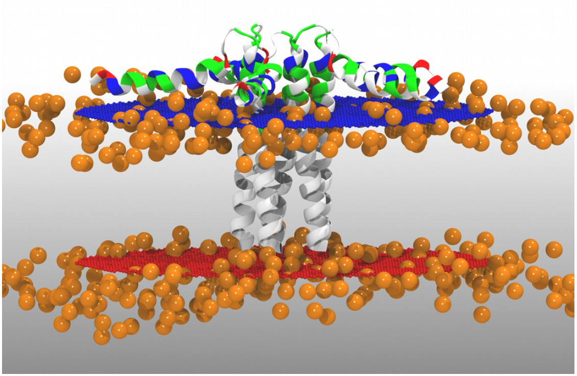
Figure 1. Protein oriented inside the membrane from the OPM database with dummy atoms represented as orange spheres.
6.1.2. Delete close contact lipid molecules
We need to use VMD to to delete lipid molecules in close contact with the protein. For a proper treatment and visualization of the system in VMD you must first generate the molecular topology and initial coordinate files.
Use pdb2gmx to convert your PDB file into GROMACS format:
gmx pdb2gmx -f 2kyv_DMPC_cg_init.pdb -o 2kyv_DMPC_cg_init.gro -p init_topol -i init_posre
When prompted, choose SIRAH force field and then SIRAH solvent models.
Caution
In GROMACS versions prior to 5.x, the “gmx” command should not be used.
CG molecules are not recognized by molecular visualizers and will not display correctly. To fix this problem you may
generate a PSF file of the system using the script g_top2psf.pl:
./sirah.ff/tools/g_top2psf.pl -i init_topol.top -o 2kyv_DMPC_cg_init.psf
Note
This is the basic usage of the script g_top2psf.pl, you can learn other capabilities from its help:
./sirah.ff/tools/g_top2psf.pl -h
Use VMD to check how the CG system looks like:
vmd 2kyv_DMPC_cg_init.psf 2kyv_DMPC_cg_init.gro -e sirah.ff/tools/sirah_vmdtk.tcl
Tip
VMD assigns default radius to unknown atom types, the script sirah_vmdtk.tcl sets the right
ones, according to the CG representation. It also provides a kit of useful selection macros, coloring methods and backmapping utilities.
Use the command sirah_help in the Tcl/Tk console of VMD to access the manual pages. To learn about SIRAH Tools’ capabilities, you can also go to the SIRAH Tools tutorial.
In the VMD main window, select Graphics > Representations. In the Selected Atoms box, type:
not (same residue as (sirah_membrane within 3.5 of sirah_protein))
To save the refined protein-membrane system, in the VMD main window click on 2kyv_DMPC_cg_init.psf, then select File > Save Coordinates. In the Selected atoms option choose the selection you have just created and Save as 2kyv_DMPC_cg.pdb.
From now on it is just normal GROMACS stuff!
6.2. PDB to GROMACS format
Use pdb2gmx to convert your PDB file into GROMACS format:
gmx pdb2gmx -f 2kyv_DMPC_cg.pdb -o 2kyv_DMPC_cg.gro
When prompted, choose SIRAH force field and then SIRAH solvent models.
Note
By default, charged terminal are used but it is possible to set them neutral with option -ter
Note
Warning messages about long, triangular or square bonds are fine and expected due to the CG topology of some residues.
Caution
However, missing atom messages are errors which probably trace back to the mapping step. In that case, check your atomistic and mapped structures and do not carry on the simulation until the problem is solved.
6.3. Solvate the system
Define the simulation box of the system
gmx editconf -f 2kyv_DMPC_cg.gro -o 2kyv_DMPC_cg_box.gro -box 12 12 12 -c
Add WT4 molecules:
gmx solvate -cp 2kyv_DMPC_cg_box.gro -cs sirah.ff/wt416.gro -o 2kyv_DMPC_cg_solv1.gro
Note
Before GROMACS version 5.x, the command gmx solvate was called genbox.
Edit the [ molecules ] section in topol.top to include the number of added WT4 molecules:
Topology before editing |
Topology after editing |
|---|---|
[ molecules ]
; Compound #mols
Protein_chain_A 1
Protein_chain_B 1
Protein_chain_C 1
Protein_chain_D 1
Protein_chain_E 1
Lipid_chain_F 1
|
[ molecules ]
; Compound #mols
Protein_chain_A 1
Protein_chain_B 1
Protein_chain_C 1
Protein_chain_D 1
Protein_chain_E 1
Lipid_chain_F 1
WT4 3875
|
Hint
If you forget to read the number of added WT4 molecules from the output of solvate, then use the following command line to get it
grep -c WP1 2kyv_DMPC_cg_solv1.gro
Caution
The number of added WT4 molecules, 3875, may change according to the software version.
Remove misplaced WT4 molecules inside the bilayer:
gmx grompp -f sirah.ff/tutorial/6/GPU/em1_CGLIPROT.mdp -p topol.top -c 2kyv_DMPC_cg_solv1.gro -o 2kyv_DMPC_cg_solv1.tpr
echo "q" | gmx make_ndx -f 2kyv_DMPC_cg_solv1.gro -o 2kyv_DMPC_cg_solv1.ndx
gmx select -f 2kyv_DMPC_cg_solv1.gro -s 2kyv_DMPC_cg_solv1.tpr -n 2kyv_DMPC_cg_solv1.ndx -on rm_close_wt4.ndx -sf sirah.ff/tutorial/6/rm_close_wt4.dat
gmx editconf -f 2kyv_DMPC_cg_solv1.gro -o 2kyv_DMPC_cg_solv2.gro -n rm_close_wt4.ndx
Caution
New GROMACS versions may complain about the non-neutral charge of the system, aborting the generation of the TPR file by command grompp. We will neutralize the system later, so to overcame this issue, just allow a warning message by adding the following keyword to the grompp command line: -maxwarn 1
Note
Consult sirah.ff/0ISSUES and FAQs for information on known solvation issues.
Edit the [ molecules ] section in topol.top to correct the number of WT4 molecules:
Hint
If you forget to read the number of added WT4 molecules from the output of solvate, then use the following command line to get it
grep -c WP1 2kyv_DMPC_cg_solv2.gro
Add CG counterions and 0.15M NaCl:
gmx grompp -f sirah.ff/tutorial/6/GPU/em1_CGLIPROT.mdp -p topol.top -c 2kyv_DMPC_cg_solv2.gro -o 2kyv_DMPC_cg_solv2.tpr
gmx genion -s 2kyv_DMPC_cg_solv2.tpr -o 2kyv_DMPC_cg_ion.gro -np 95 -pname NaW -nn 110 -nname ClW
When prompted, choose to substitute WT4 molecules by ions.
Note
The available electrolyte species in SIRAH force field are: Na⁺ (NaW), K⁺ (KW) and Cl⁻ (ClW) which represent solvated ions in solution. One ion pair (e.g., NaW-ClW) each 34 WT4 molecules results in a salt concentration of ~0.15M (see Appendix for details). Counterions were added according to Machado et al..
Edit the [ molecules ] section in topol.top to include the CG ions and the correct number of WT4.
Before running the simulation it may be a good idea to visualize your molecular system. CG molecules are not recognized by molecular visualizers and will not display correctly. To fix this problem you may
generate a PSF file of the system using the script g_top2psf.pl:
./sirah.ff/tools/g_top2psf.pl -i topol.top -o 2kyv_DMPC_cg_ion.psf
Note
This is the basic usage of the script g_top2psf.pl, you can learn other capabilities from its help:
./sirah.ff/tools/g_top2psf.pl -h
Use VMD to check how the CG system looks like:
vmd 2kyv_DMPC_cg_ion.psf 2kyv_DMPC_cg_ion.gro -e sirah.ff/tools/sirah_vmdtk.tcl
Tip
VMD assigns default radius to unknown atom types, the script sirah_vmdtk.tcl sets the right ones, according to the CG representation. It also provides a kit of useful selection macros, coloring methods and backmapping utilities.
Use the command sirah_help in the Tcl/Tk console of VMD to access the manual pages. To learn about SIRAH Tools’ capabilities, you can also go to the SIRAH Tools tutorial.
6.4. Generate position restraint files
To achive a proper interaction between the protein and bilayer, we will perform a equilibration step applying restraints over the protein backbone and lipids’ phosphate groups.
Important
GROMACS enumerates atoms starting from 1 in each topology file (e.i. topol_*.itp). In order to avoid atom index discordance between the .gro file of the system and each topology, we will need independent .gro files for the PLN monomer and the DMPC bilayer.
Crate an index file of the system with a group for PLN monomer, then generate the .gro file of it.
Note
WT4 and CG ions (NaW, ClW) are automatically set to the group SIRAH-Solvent while DMPC (named CMM at CG level) is assigned to group Lipid.
echo -e "ri 1-52\nq" | gmx make_ndx -f 2kyv_DMPC_cg_ion.gro -o 2kyv_DMPC_cg_ion.ndx
gmx editconf -f 2kyv_DMPC_cg_ion.gro -n 2kyv_DMPC_cg_ion.ndx -o 2kyv_DMPC_cg_monomer.gro
When prompted, choose r_1-52.
Create an index file for the monomer and add a group for the backbone GO and GN beads.
echo -e "a GO GN \nq" | gmx make_ndx -f 2kyv_DMPC_cg_monomer.gro -o 2kyv_DMPC_cg_monomer.ndx
Create a position restraint file for the monomer backbone.
gmx genrestr -f 2kyv_DMPC_cg_monomer.gro -n 2kyv_DMPC_cg_monomer.ndx -fc 100 100 100 -o posre_BB.itp
When prompted, choose GO_GN.
Edit each topol_Protein_chain_*.itp (A to E) to include the new position restraints:
Topology before editing |
Topology after editing |
|---|---|
; Include Position restraint file
#ifdef POSRES
#include "posre_Protein.itp"
#endif
|
; Include Position restraint file
#ifdef POSRES
#include "posre_Protein.itp"
#endif
#ifdef POSREBB
#include "posre_BB.itp"
#endif
|
Use a similar procedure to set the positional restraints on lipid’s phosphates.
gmx editconf -f 2kyv_DMPC_cg_ion.gro -n 2kyv_DMPC_cg_ion.ndx -o DMPC_cg.gro
When prompted, choose Lipid.
Create an index file of the membrane and add a group for phosphates (BFO beads).
echo -e "a BFO \nq" | gmx make_ndx -f DMPC_cg.gro -o DMPC_cg.ndx
Create a position restraint file for phosphate groups in z coordinate.
gmx genrestr -f DMPC_cg.gro -n DMPC_cg.ndx -fc 0 0 100 -o posre_Pz.itp
When prompted, choose BFO.
Edit topol_Lipid_chain_F.itp to include the new position restraints and define the flags POSREZ to switch on these restraints in the input file (.mdp).
Topology before editing |
Topology after editing |
|---|---|
; Include Position restraint file
#ifdef POSRES
#include "posre_Lipid_chain_F.itp"
#endif
|
; Include Position restraint file
#ifdef POSRES
#include "posre_Lipid_chain_F.itp"
#endif
#ifdef POSREZ
#include "posre_Pz.itp"
#endif
|
6.5. Run the simulation
Important
By default, in this tutorial we will use input files for GROMACS on GPU (sirah.ff/tutorial/6/GPU). Example input files for using GROMACS on CPU can be found at: sirah.ff/tutorial/6/CPU.
The folder sirah.ff/tutorial/6/GPU/ contains typical input files for energy minimization
(em1_CGLIPROT.mdp and em2_CGLIPROT.mdp), equilibration (eq1_CGLIPROT.mdp and eq2_CGLIPROT.mdp) and production (md_CGLIPROT.mdp) runs. Please
check carefully the input flags therein.
Make a new folder for the run:
mkdir run; cd run
Energy Minimization of side chains by restraining the backbone:
gmx grompp -f ../sirah.ff/tutorial/6/GPU/em1_CGLIPROT.mdp -p ../topol.top -n ../2kyv_DMPC_cg_ion.ndx -c ../2kyv_DMPC_cg_ion.gro -r ../2kyv_DMPC_cg_ion.gro -o 2kyv_DMPC_cg_em1.tpr
gmx mdrun -deffnm 2kyv_DMPC_cg_em1 &> EM1.log &
Energy Minimization of the whole system:
gmx grompp -f ../sirah.ff/tutorial/6/GPU/em2_CGLIPROT.mdp -p ../topol.top -n ../2kyv_DMPC_cg_ion.ndx -c 2kyv_DMPC_cg_em1.gro -r 2kyv_DMPC_cg_em1.gro -o 2kyv_DMPC_cg_em2.tpr
gmx mdrun -deffnm 2kyv_DMPC_cg_em2 &> EM2.log &
Equilibration 1:
Warning
Some large systems may turn unstable. In this case set fourierspacing to 0.12 in the mdp files.
Position restraints are defined in eq1_CGLIPROT.mdp file for protein backbone in xyz and phosphate groups (BFO beads) in z coordinate by setting keywords -DPOSREBB and -DPOSREZ, respectively.
gmx grompp -f ../sirah.ff/tutorial/6/GPU/eq1_CGLIPROT.mdp -p ../topol.top -n ../2kyv_DMPC_cg_ion.ndx -c 2kyv_DMPC_cg_em2.gro -r 2kyv_DMPC_cg_em2.gro -o 2kyv_DMPC_cg_eq1.tpr
gmx mdrun -deffnm 2kyv_DMPC_cg_eq1 &> EQ1.log &
Equilibration 2:
gmx grompp -f ../sirah.ff/tutorial/6/GPU/eq2_CGLIPROT.mdp -p ../topol.top -n ../2kyv_DMPC_cg_ion.ndx -c 2kyv_DMPC_cg_eq1.gro -r 2kyv_DMPC_cg_eq1.gro -o 2kyv_DMPC_cg_eq2.tpr
gmx mdrun -deffnm 2kyv_DMPC_cg_eq2 &> EQ2.log &
Production (1000ns):
gmx grompp -f ../sirah.ff/tutorial/6/GPU/md_CGLIPROT.mdp -p ../topol.top -n ../2kyv_DMPC_cg_ion.ndx -c 2kyv_DMPC_cg_eq2.gro -r 2kyv_DMPC_cg_eq2.gro -o 2kyv_DMPC_cg_md.tpr
gmx mdrun -deffnm 2kyv_DMPC_cg_md &> MD.log &
6.6. Visualizing the simulation
That’s it! Now you can analyze the trajectory.
Process the output trajectory at folder run/ to account for the Periodic Boundary Conditions (PBC):
gmx trjconv -s 2kyv_DMPC_cg_em1.tpr -f 2kyv_DMPC_cg_md.xtc -o 2kyv_DMPC_cg_md_pbc.xtc -n ../2kyv_DMPC_cg_ion.ndx -pbc mol
When prompted, choose System for output.
Now you can check the simulation using VMD:
vmd ../2kyv_DMPC_cg_ion.psf ../2kyv_DMPC_cg_ion.gro 2kyv_DMPC_cg_md_pbc.xtc -e ../sirah.ff/tools/sirah_vmdtk.tcl
Note
The file sirah_vmdtk.tcl is a Tcl script that is part of SIRAH Tools and contains the macros to properly visualize the coarse-grained structures in VMD. Use the command sirah_help in the Tcl/Tk console of VMD to access the manual pages. To learn about SIRAH Tools’ capabilities, you can also go to the SIRAH Tools tutorial.
7. SMD with multiscale solvent
Note
Please report bugs, errors or enhancement requests through Issue Tracker or if you have a question about SIRAH open a New Discussion.
This tutorial shows how to apply the multiscale solvation approach of SIRAH force field in Steered Molecular Dynamics (SMD) simulations. In this tutorial, an immunoglobulin domain known as I10 derived from Titin is enclosed by CG waters referred to as WatFour (WT4). These waters are further embedded within supra-coarse-grained (SCG) molecules called WatElse (WLS), which serve as a representation of bulk water. The main references for this tutorial are: Darré et al. and Machado et al..
Note
We strongly advise you to read and complete Tutorial 2 and Tutorial 3 before starting. We also recommend you to perform the Umbrella Sampling tutorial of GROMACS to get familiar with pulling simulations parameters.
Important
Check the Setting up SIRAH section for download and set up details before starting this tutorial.
Since this is Tutorial 7, remember to replace X.X, the files corresponding to this tutorial can be found in: sirah.ff/tutorial/7/
7.1. Setting pulling direction
Caution
The basic idea behind SMD is to apply an external force or mechanical perturbation to a specific part of the biomolecular system under study and observe its response. This external force is applied to one atom or groups of atoms as a “steering” force, guiding or pulling the atoms along a predefined path or direction. Thus, prior to proceeding, we need to remember to prepare the PDB file to specify the pulling direction. In this example, the Z-axis was employed to orient the protein terminus and to determine the box size.
In sirah_[version].ff/tutorial/7/ you will find the I10 domain (PDB code: 4QEG) already aligned along the Z-axis, I10_z.pdb file.
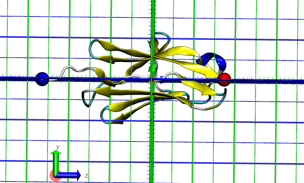
Figure 1. I10 domain N-terminal (blue) and C-terminal (red) aligned to the Z-axis from I10_z.pdb.
To get the protein aligned along the Z-axis, we used the following commands in VMD’s Tk Console (Extensions > Tk Console):
#Select the protein
set all [atomselect top "protein"]

#Change protein coordinates to align to its center
$all moveby  [vecinvert [measure center $all]]

#Rotate around x-axis 50 degrees
$all move [transaxis x 50]

#Rotate around y-axis -11 degrees
$all move [transaxis y -11]

#Write PDB file with the protein aligned to z-axis
$all writepdb I10_z.pdb
Note
For setting up your own system you can open your own PDB in VMD and probe different alternatives to get the correct direction.
7.2. Build CG representations
Caution
The mapping to CG requires the correct protonation state of each residue at a given pH. We recommend using the CHARMM-GUI server and use the PDB Reader & Manipulator to prepare your system. An account is required to access any of the CHARMM-GUI Input Generator modules, and it can take up to 24 hours to obtain one.
Other option is the PDB2PQR server and choosing the output naming scheme of AMBER for best compatibility. This server was utilized to generate the PQR file featured in this tutorial. Be aware that modified residues lacking parameters such as: MSE (seleno MET), TPO (phosphorylated THY), SEP (phosphorylated SER) or others are deleted from the PQR file by the server. In that case, mutate the residues to their unmodified form before submitting the structure to the server.
See Tutorial 3 for cautions while preparing and mapping atomistic proteins to SIRAH.
Important
Check the Setting up SIRAH section for download and set up details before starting this tutorial.
Since this is Tutorial 7, remember to replace X.X, the files corresponding to this tutorial can be found in: sirah.ff/tutorial/7/
Map the atomistic structure of the I10 domain to its CG representation:
./sirah.ff/tools/CGCONV/cgconv.pl -i sirah.ff/tutorial/7/I10_z.pqr -o I10_cg.pdb
The input file -i I10_z.pqr contains the atomistic representation of 4QEG structure at pH 7.0 and aligned to the Z-axis, while the output -o I10_cg.pdb is its SIRAH CG representation.
Tip
This is the basic usage of the script cgconv.pl, you can learn other capabilities from its help by typing:
./sirah.ff/tools/CGCONV/cgconv.pl -h
Please check both PDB and PQR structures using VMD:
vmd -m sirah.ff/tutorial/7/I10_z.pqr I10_cg.pdb
From now on it is just normal GROMACS stuff!
7.3. PDB to GROMACS format
Use pdb2gmx to convert your PDB file into GROMACS format:
gmx pdb2gmx -f I10_cg.pdb -o I10_cg.gro
When prompted, choose SIRAH force field and then SIRAH solvent models. In this specific case, the charge of the system is -5.000 e; this will be addressed later.
Note
By default charged terminal are used but it is possible to set them neutral with option -ter.
Note
Warning messages about long, triangular or square bonds are fine and expected due to the CG topology of some residues.
Caution
However, missing atom messages are errors which probably trace back to the mapping step. In that case, check your atomistic and mapped structures and do not carry on the simulation until the problem is solved.
7.4. Solvate the system
Danger
Since we are doing a SMD simulation, we need to carefully set the box dimensions to provide enough solvent to the “stretched” protein and keep a good separation between the surfaces of periodic images.
In this system, I10 has 88 amino acids and the maximum extension size of each amino acid is 0.34 nm. Thus, “stretched” protein will be 88 * 0.34 = 29.92 nm (~ 30.0 nm) long. In order to accommodate the pulling, GROMACS stipulates a minimum box size double this value, i.e. 60 nm for the Z-axis. However, for optimal results, it is recommended that the dimensions of the box be 2.5 to 3 times greater than the maximum length of the protein when in its extended conformation. Therefore, for this tutorial the box used is 10 10 90 nm.
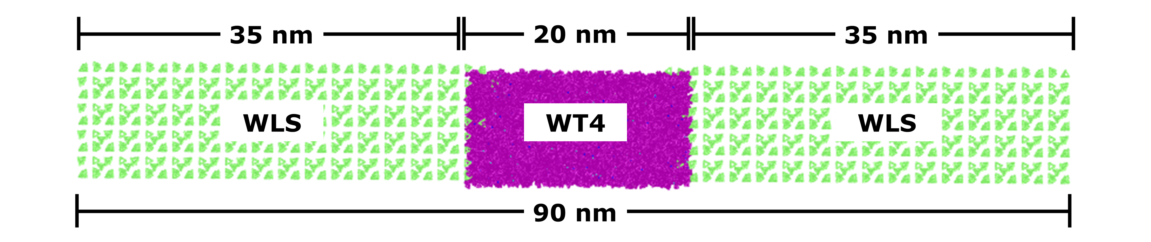
Figure 2. Dimensions of the multiscale solvation box used in this tutorial.
In order to have a multiscale solvent approach using WT4 (CG solvent) and WLS (Supra-CG solvent), two steps are needed to solvate the systems.
First, define the simulation region of the system to be enclosed by WT4 (purple in Figure 2)
gmx editconf -f I10_cg.gro -o I10_cg_box.gro -box 10 10 20 -bt triclinic -c
Note
At this step, if you don’t want to use a multiscale solvent method, the whole box dimension (10 10 90 nm) can be used to add only WT4 molecules.
Add WT4 molecules:
gmx solvate -cp I10_cg_box.gro -cs sirah.ff/wt416.gro -o I10_cg_solv1.gro
Note
Before GROMACS version 5.x, the command gmx solvate was called genbox.
Edit the [ molecules ] section in topol.top to include the number of added WT4 molecules:
Topology before editing |
Topology after editing |
|---|---|
[ molecules ]
; Compound #mols
Protein_chain_A 1
|
[ molecules ]
; Compound #mols
Protein_chain_A 1
WT4 6281
|
Hint
If you forget to read the number of added WT4 molecules from the output of solvate, then use the following command line to get it:
grep -c WP1 I10_cg_solv1.gro
Caution
The number of added WT4 molecules, 6281, may change according to the software version.
Remove misplaced WT4 molecules within 0.3 nm of protein:
echo q | gmx make_ndx -f I10_cg_solv1.gro -o I10_cg_solv1.ndx
gmx grompp -f sirah.ff/tutorial/7/em1_CGPROT.mdp -p topol.top -po delete1.mdp -c I10_cg_solv1.gro -o I10_cg_solv1.tpr -maxwarn 2
Caution
New GROMACS versions may complain about not used macros and the non-neutral charge of the system, aborting the generation of the TPR file by command grompp. We will neutralize the system later, so to overcame these issues, just allow warning messages by adding the following keyword to the grompp command line: -maxwarn 2
gmx select -f I10_cg_solv1.gro -s I10_cg_solv1.tpr -n I10_cg_solv1.ndx -on rm_close_wt4.ndx -select 'not (same residue as (resname WT4 and within 0.3 of group Protein))'
gmx editconf -f I10_cg_solv1.gro -o I10_cg_solv2.gro -n rm_close_wt4.ndx
Edit the [ molecules ] section in topol.top to correct the number of WT4 molecules, 6261.
Hint
If you forget to read the number of added WT4 molecules from the output of solvate, then use the following command line to get it:
grep -c WP1 I10_cg_solv2.gro
Now, we include the second solvent layer of solvent with WLS molecules (green in Figure 2):
gmx editconf -f I10_cg_solv2.gro -o I10_cg_box2.gro -box 10 10 90 -bt triclinic -c
Hint
We can check the final box dimensions with VMD:
vmd I10_cg_box2.gro
In the Tk Console (Extensions > Tk Console) use the command:
pbc box
Add WLS molecules:
gmx solvate -cp I10_cg_box2.gro -cs sirah.ff/wlsbox.gro -o I10_cg_solv3.gro
Note
Before GROMACS version 5.x, the command gmx solvate was called genbox.
Edit the [ molecules ] section in topol.top to include the number of added WLS molecules:
Topology before editing |
Topology after editing |
|---|---|
[ molecules ]
; Compound #mols
Protein_chain_A 1
WT4 6261
|
[ molecules ]
; Compound #mols
Protein_chain_A 1
WT4 6261
WLS 4697
|
Hint
If you forget to read the number of added WLS molecules from the output of solvate, then use the following command line to get it:
grep -c LN1 I10_cg_solv3.gro
Caution
The number of added WLS molecules, 4697, may change according to the software version.
Remove misplaced WLS molecules within 7.8 nm of protein:
echo q | gmx make_ndx -f I10_cg_solv3.gro -o I10_cg_solv3.ndx
gmx grompp -f sirah.ff/tutorial/7/em1_CGPROT.mdp -p topol.top -po delete3.mdp -c I10_cg_solv3.gro -o I10_cg_solv3.tpr -maxwarn 2
Caution
New GROMACS versions may complain about not used macros and the non-neutral charge of the system, aborting the generation of the TPR file by command grompp. We will neutralize the system later, so to overcame this issue, just allow warning messages by adding the following keyword to the grompp command line: -maxwarn 2
gmx select -f I10_cg_solv3.gro -s I10_cg_solv3.tpr -n I10_cg_solv3.ndx -on rm_close_wls.ndx -select 'not (same residue as (resname WLS and within 7.8 of group Protein))'
gmx editconf -f I10_cg_solv3.gro -o I10_cg_solv4.gro -n rm_close_wls.ndx
Edit the [ molecules ] section in topol.top to correct the number of WLS molecules, 4580.
Hint
If you forget to read the number of added WLS molecules from the output of solvate, then use the following command line to get it
grep -c LN1 I10_cg_solv4.gro
Note
Consult sirah.ff/0ISSUES and FAQs for information on known solvation issues.
Add CG counterions and 0.15M NaCl:
gmx grompp -f sirah.ff/tutorial/7/em1_CGPROT.mdp -p topol.top -po delete4.mdp -c I10_cg_solv4.gro -o I10_cg_solv4.tpr -maxwarn 2
Caution
New GROMACS versions may complain about not used macros and the non-neutral charge of the system, aborting the generation of the TPR file by command grompp. We are about to neutralize the system, so to overcame this issue, just allow warning messages by adding the following keyword to the grompp command line: -maxwarn 2
gmx genion -s I10_cg_solv4.tpr -o I10_cg_ion.gro -np 189 -pname NaW -nn 184 -nname ClW
When prompted, choose to substitute WT4 molecules by ions.
Note
The available electrolyte species in SIRAH force field are: Na⁺ (NaW), K⁺ (KW) and Cl⁻ (ClW) which represent solvated ions in solution. One ion pair (e.g., NaW-ClW) each 34 WT4 molecules results in a salt concentration of ~0.15M (see Appendix for details). Counterions were added according to Machado et al..
Edit the [ molecules ] section in topol.top to include the CG ions and the correct number of WT4, WLS, and ions.
Topology before editing |
Topology after editing |
|---|---|
[ molecules ]
; Compound #mols
Protein_chain_A 1
WT4 6261
WLS 4582
|
[ molecules ]
; Compound #mols
Protein_chain_A 1
WT4 5888
NaW 189
ClW 184
WLS 4580
|
Caution
Following the above order is important: the number of WT4 comes first, then the number of ions, and finally WLS.
Before running the simulation it may be a good idea to visualize your molecular system. CG molecules are not recognized by molecular visualizers and will not display correctly. To fix this problem you may
generate a PSF file of the system using the script g_top2psf.pl:
./sirah.ff/tools/g_top2psf.pl -i topol.top -o I10_cg_ion.psf
Note
This is the basic usage of the script g_top2psf.pl, you can learn other capabilities from its help:
./sirah.ff/tools/g_top2psf.pl -h
Use VMD to check how the CG system looks like:
vmd I10_cg_ion.psf I10_cg_ion.gro -e sirah.ff/tools/sirah_vmdtk.tcl
Tip
VMD assigns default radius to unknown atom types, the script sirah_vmdtk.tcl sets the right ones, according to the CG representation. It also provides a kit of useful selection macros, coloring methods and backmapping utilities.
Use the command sirah_help in the Tcl/Tk console of VMD to access the manual pages. To learn about SIRAH Tools’ capabilities, you can also go to the SIRAH Tools tutorial.
To achive a proper interaction between the protein and solvent, we will perform a equilibration step applying restraints over the protein backbone.
Create an index file including a group for the backbone GN and GO beads:
echo -e "a GN GO\n\nq" | gmx make_ndx -f I10_cg_ion.gro -o I10_cg_ion.ndx
Note
WT4 and CG ions (NaW, ClW) are automatically set to the group SIRAH-Solvent.
Generate restraint files for the backbone GN and GO beads:
gmx genrestr -f I10_cg.gro -n I10_cg_ion.ndx -o bkbres.itp
When prompted, choose the group GN_GO.
gmx genrestr -f I10_cg.gro -n I10_cg_ion.ndx -o bkbres_soft.itp -fc 100 100 100
Here, choose the group GN_GO.
Add the restraints to topol.top:
Topology before editing |
Topology after editing |
|---|---|
; Include Position restraint file
#ifdef POSRES
#include "posre.itp"
#endif
; Include water topology
#include "../sirah.ff/solv.itp"
#ifdef POSRES_WATER
; Position restraint for each water oxygen
[ position_restraints ]
; i funct fcx fcy fcz
1 1 1000 1000 1000
#endif
|
; Include Position restraint file
#ifdef POSRES
#include "posre.itp"
#endif
; Backbone restraints
#ifdef GN_GO
#include "bkbres.itp"
#endif
; Backbone soft restrains
#ifdef GN_GO_SOFT
#include "bkbres_soft.itp"
#endif
; Include water topology
#include "../sirah.ff/solv.itp"
#ifdef POSRES_WATER
; Position restraint for each water oxygen
[ position_restraints ]
; i funct fcx fcy fcz
1 1 1000 1000 1000
#endif
|
7.5. Run the simulation
Important
By default in this tutorial we will use input files for GROMACS on GPU (sirah.ff/tutorial/7/).
The folder sirah.ff/tutorial/7/ contains typical input files for energy minimization (em1_CGPROT.mdp, em2_CGPROT.mdp, and em3_CGPROT.mdp), equilibration (eq1_CGPROT.mdp and eq2_CGPROT.mdp), production (md_CGPROT.mdp) and SMD (SMD_Force_CGPROT.mdp and SMD_Velocity_CGPROT.mdp) runs. Please check carefully the input flags therein.
Make a new folder for the run:
mkdir run; cd run
Energy Minimization of side chains and Sirah-solvent by restraining the backbone:
gmx grompp -f ../sirah.ff/tutorial/7/em1_CGPROT.mdp -p ../topol.top -po em1.mdp -n ../I10_cg_ion.ndx -c ../I10_cg_ion.gro -r ../I10_cg_ion.gro -o I10_cg_em1.tpr
gmx mdrun -deffnm I10_cg_em1 &> EM1.log &
Energy Minimization of side chains by restraining the backbone:
gmx grompp -f ../sirah.ff/tutorial/7/em2_CGPROT.mdp -p ../topol.top -po em2.mdp -n ../I10_cg_ion.ndx -c I10_cg_em1.gro -r I10_cg_em1.gro -o I10_cg_em2.tpr
gmx mdrun -deffnm I10_cg_em2 &> EM2.log &
Energy Minimization of whole system:
gmx grompp -f ../sirah.ff/tutorial/7/em3_CGPROT.mdp -p ../topol.top -po em3.mdp -n ../I10_cg_ion.ndx -c I10_cg_em2.gro -o I10_cg_em3.tpr
gmx mdrun -deffnm I10_cg_em3 &> EM3.log &
Solvent equilibration:
gmx grompp -f ../sirah.ff/tutorial/7/eq1_CGPROT.mdp -p ../topol.top -po eq1.mdp -n ../I10_cg_ion.ndx -c I10_cg_em2.gro -r I10_cg_em2.gro -o I10_cg_eq1.tpr
gmx mdrun -deffnm I10_cg_eq1 &> EQ1.log &
Soft equilibration to improve side chain solvation:
gmx grompp -f ../sirah.ff/tutorial/7/eq2_CGPROT.mdp -p ../topol.top -po eq2.mdp -n ../I10_cg_ion.ndx -c I10_cg_eq1.gro -r I10_cg_eq1.gro -o I10_cg_eq2.tpr
gmx mdrun -deffnm I10_cg_eq2 &> EQ2.log &
SMD Force or velocity:
Here, we need to modify the index file to add the “Pull” groups, before running SMD force or velocity simulations.
Copy the I10_cg_ion.ndx with a new name:
cp ../I10_cg_ion.ndx ../I10_cg_ion_pull.ndx
Open the I10_cg_ion_pull.ndx in any text editor and manually add to the end of the I10_cg_ion_pull.ndx file these two new groups:
Groups to add |
|---|
[ pull1 ]
4
[ pull2 ]
437
|
In this tutorial we are going to run only the SMD Force simulation:
gmx grompp -f ../sirah.ff/tutorial/7/SMD_Force_CGPROT.mdp -p ../topol.top -po md.mdp -n ../I10_cg_ion_pull.ndx -c I10_cg_eq2.gro -o I10_cg_SMD_F.tpr
gmx mdrun -deffnm I10_cg_SMD_F &> SMD_F.log &
However, you can also run a SMD Velocity simulation:
gmx grompp -f ../sirah.ff/tutorial/7/SMD_Velocity_CGPROT.mdp -p ../topol.top -po md.mdp -n ../I10_cg_ion_pull.ndx -c I10_cg_eq2.gro -o I10_cg_SMD_V.tpr
gmx mdrun -deffnm I10_cg_SMD_V &> SMD_V.log &
Note
It is also possible to use the files you made to run a MD simulation of your system:
Production (1000ns):
gmx grompp -f ../sirah.ff/tutorial/7/md_CGPROT.mdp -p ../topol.top -po md.mdp -n ../I10_cg_ion.ndx -c I10_cg_eq2.gro -o I10_cg_md.tpr
gmx mdrun -deffnm I10_cg_md &> MD.log &
7.6. Visualizing the simulation
That’s it! Now you can analyze the trajectory.
GROMACS automatically creates plot results to the SMD simulations. The position versus simulation time is saved as I10_cg_md_pullx.xvg, and the force versus simulation time is saved as I10_cg_md_pullf.xvg.
You can plot the results using Xmgrace.
xmgrace I10_cg_md_pullx.xvg
For I10_cg_md_pullx.xvg, a plot similar to Figure 3 will appear:
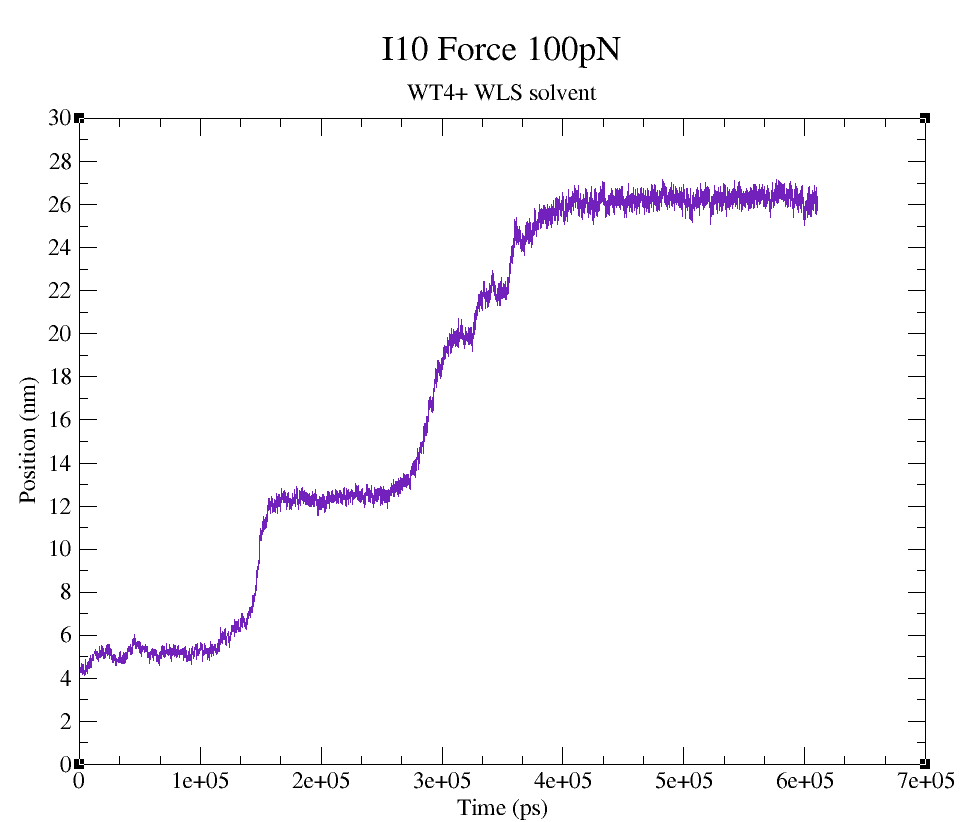
Figure 3. Position vs Time plot created by GROMACS from the SMD simulation.
In addition, you can process the output trajectory at folder run/ to account for the Periodic Boundary Conditions (PBC).
For SMD Force:
gmx trjconv -s I10_cg_em1.tpr -f I10_cg_SMD_F.xtc -o I10_cg_SMD_F_pbc.xtc -n ../I10_cg_ion_pull.ndx -ur compact -center -pbc mol
For SMD Velocity:
gmx trjconv -s I10_cg_em1.tpr -f I10_cg_SMD_V.xtc -o I10_cg_SMD_V_pbc.xtc -n ../I10_cg_ion_pull.ndx -ur compact -center -pbc mol
When prompted, choose Protein for centering and System for output.
Note
If you had also run a MD simulation, you could use the following commands to account for PBC:
gmx trjconv -s I10_cg_em1.tpr -f I10_cg_md.xtc -o I10_cg_md_pbc.xtc -n ../I10_cg_ion.ndx -ur compact -center -pbc mol
Now you can check the simulation using VMD:
vmd ../I10_cg_ion.psf ../I10_cg_ion.gro I10_cg_SMD_F_pbc.xtc -e ../sirah.ff/tools/sirah_vmdtk.tcl
Note
The file sirah_vmdtk.tcl is a Tcl script that is part of SIRAH Tools and contains the macros to properly visualize the coarse-grained structures in VMD. Use the command sirah_help in the Tcl/Tk console of VMD to access the manual pages. To learn about SIRAH Tools’ capabilities, you can also go to the SIRAH Tools tutorial.